Introduction
If you are a researcher in academia or industry, depending where you are in your causal journey, this post may blow your mind! Its primary purpose is to convey that if you have not started thinking about causality yet, then you should perhaps start to feel deep existential dread.
Let’s say you are doing a social science study and you are interested in how a bunch of predictor variables (e.g. impulsivity, age, sex, etc.) influence some outcome variable such as body mass index. An exceedingly common practice is to throw all of these variables into a multiple linear regression.
When you do this you will get regression coefficients that inform you of the statistical associations between your predictors and outcome variables. The problem is that these are only sometimes useful in telling us what we really care about, namely the causal relationships between the variables.
Now, it’s entirely possible that you’ve gotten lucky and by running a multiple regression with a bunch of control variables you end up with a statistical estimate that is not too far away from a true causal effect.
Then again, it is entirely possible that you are not lucky, and by including one or more predictor variables in your regression you have actually introduced massive bias into your estimate of the causal effect. Maybe you think there is a causal effect \(X \rightarrow Y\) but actually there is no causal effect at all. Or maybe there is a causal effect but it is in the opposite direction to what you think. Or maybe there is a causal effect but it is much larger or smaller than you think.
At this point you might be thinking either “I don’t believe you” or “I need to be convinced before I start to panic.” Well, that is what this post is about. By using a simulated dataset with a known causal structure, we will see how different approaches to estimating causal effects can lead to very different results.
We will see two approaches that can be used to estimate causal effects: (1) linear regression (with good controls included and none of the bad controls), and (2) structural causal models. The first approach is perhaps easier to implement because regressions are familiar, but the second approach is more powerful and automatic. But there is no magic pill however, both approaches require you to think carefully about the causal structure of your data, and there are no guarantees that you’ve imagined the correct causal structure. But by at least thinking about it we can do our best to avoid making egregious errors out of ignorance.
Generate a dataset
First we will generate some data from this causal DAG. Just to keep things simple, all the nodes are normally distributed and the relationships between the nodes are linear.
Let’s generate a simulated dataset of 5,000 observations and look at the first 5. This is perhaps quite a lot of observations, but doing this means that we can be less worried about the estimation error and focus more on how good or bad our estimates are in the best case scenario of abundant data.
Code
N = 5_000
Q = rng.normal(size=N)
X = rng.normal(loc=0.14*Q, scale=0.4, size=N)
Y = rng.normal(loc=0.7*X + 0.11*Q, scale=0.24, size=N)
P = rng.normal(loc=0.43*X + 0.21*Y, scale=0.22, size=N)
df = pd.DataFrame({"Q": Q, "X": X, "Y": Y, "P": P})

df.head()| Q | X | Y | P | |
|---|---|---|---|---|
| 0 | 0.304717 | -0.060520 | 0.033461 | 0.185277 |
| 1 | -1.039984 | -0.265392 | -0.084383 | 0.079660 |
| 2 | 0.750451 | -0.173601 | -0.392316 | 0.007946 |
| 3 | 0.940565 | 0.303072 | 0.247141 | 0.279045 |
| 4 | -1.951035 | -0.179286 | -0.141118 | -0.015906 |
Importantly for later, we specified a true causal effect between \(X \rightarrow Y\) of 0.7. We will see how well we can recover this value with different approaches below.
Linear regression approach
Approach 1: estimate \(X \rightarrow Y\) only.
What we care about is the relationship between \(X\) and \(Y\). This might be a bit simplistic, but it is not uncommon to see people just estimate this relationship directly. We can build a model to do this in bambi (Capretto et al. 2022) using trusty formula notation, Y ~ X (Wilkinson and Rogers 1973).
model = bmb.Model('Y ~ X', df)
results = model.fit(random_seed=RANDOM_SEED)
We can use the arviz package (Kumar et al. 2019) to plot the posterior distribution of the causal effect of \(X \rightarrow Y\). For the non-Bayesians, you can think of this as the distribution of relative credibility of different causal effect strengths given the data and the model.
Code
ax = az.plot_posterior(results.posterior["X"], ref_val=0.7)
ax.set_title(r"Posterior distribution of causal effect of $X \rightarrow Y$");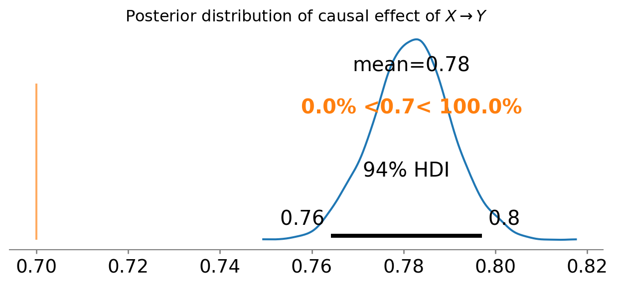
Okay, so this didn’t work out too well1. We can see that our estimated causal influence of \(X \rightarrow Y\) is way off the true value. Most people with some statistical training won’t be too surprised by this. After all, we did not take into account any of the other variables in our dataset.
Approach 2 - include all the variables in the multiple regression
So let’s try to fix that. This time we will include all the variables in the regression. This is a very common approach and one that I used many times in my academic research career. The approach has been termed “the causal salad” (see McElreath 2020; also Bulbulia et al. 2021). The intuition is that if we include all the variables into the regression and then we can see the effect of \(X\) on \(Y\) after controlling for all the other variables. Kind of makes sense right? But let’s see how well that works out for us.
model = bmb.Model('Y ~ Q + X + P', df)
results = model.fit(random_seed=RANDOM_SEED)
Code
ax = az.plot_posterior(results.posterior["X"], ref_val=0.7)
ax.set_title(r"Posterior distribution of causal effect of $X \rightarrow Y$");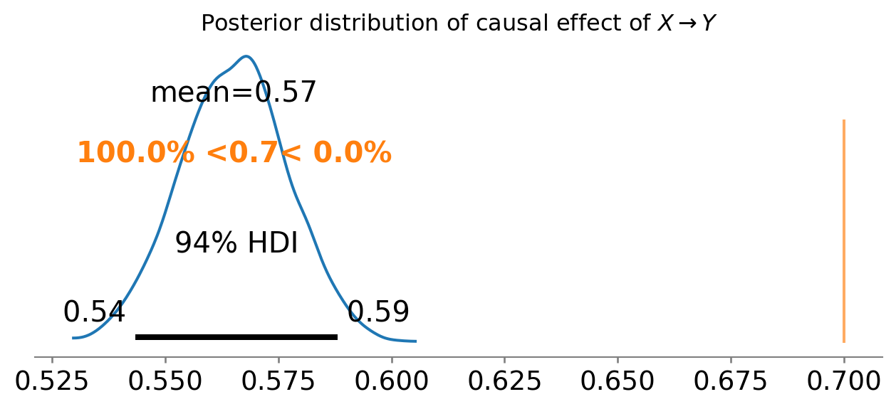
Arrrrrrggggghhhh! This is even worse than before. What is going on here? Well, the problem is that we have included both good and bad controls in our regression.
Good and bad controls? What are you talking about? Many people will not have heard of this before. I certainly hadn’t until I started reading about causal inference.
Approach 3 - include only the good controls
So I’m not going to really explain how you find out what the good controls are. That is a whole other topic. For now, all you need to know is that we have a backdoor path between \(X\) and \(Y\) via \(Q\). What this means is that there is a statistical route in which \(X\) can influence \(Y\) via \(Q\). When we have a backdoor path, we need to block it. We can do this by including \(Q\) in our regression. This is a good control.
model = bmb.Model('Y ~ X + Q', df)
results = model.fit(random_seed=RANDOM_SEED)
Code
ax = az.plot_posterior(results.posterior["X"], ref_val=0.7)
ax.set_title(r"Posterior distribution of causal effect of $X \rightarrow Y$");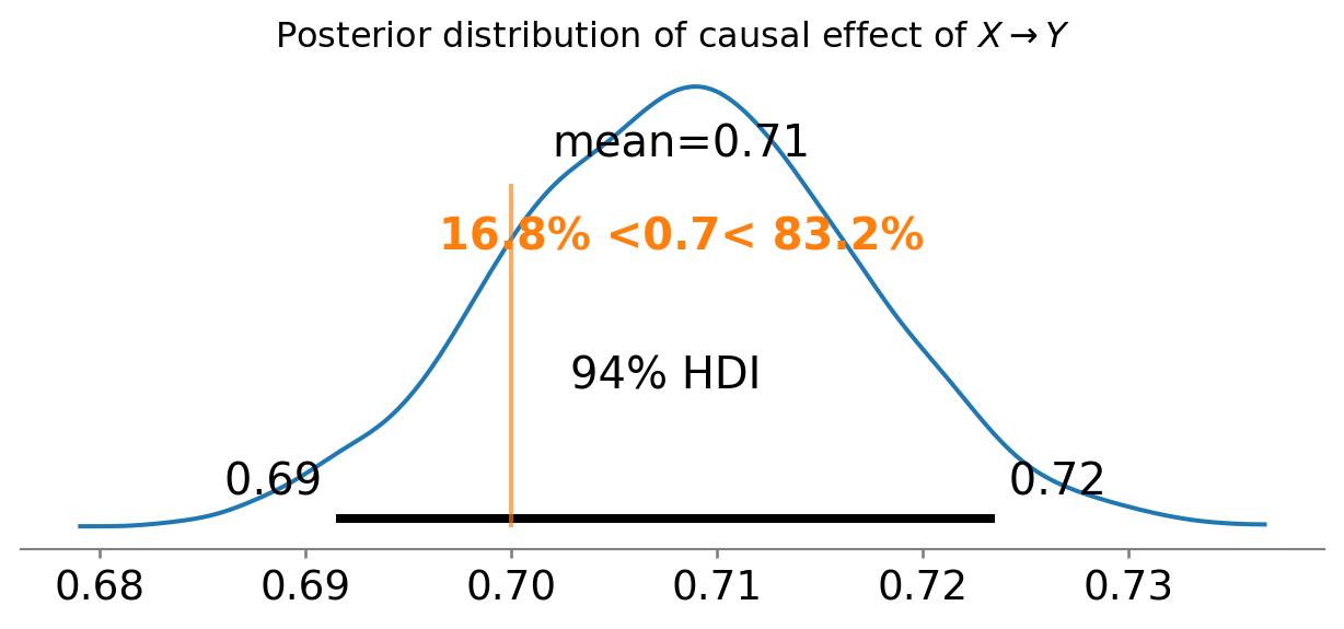
Sweet! We have recovered the true causal effect of \(X \rightarrow Y\). We did this through the ‘magic’ of only including the good controls in our regression.
Bayesian Structural Causal Modeling approach
But what if we don’t want to do all that? What if we just want to specify the DAG and let the Bayes do the rest?
Well, let’s do that. First we will specify the DAG using the PyMC (Wiecki et al. 2023) package and plot its graphical representation.
Code
with pm.Model() as model:
    # data
    _Q = pm.MutableData("_Q", df["Q"])
    _X = pm.MutableData("_X", df["X"])
    _Y = pm.MutableData("_Y", df["Y"])
    _P = pm.MutableData("_P", df["P"])

    # priors on slopes
    # x ~ q
    qx = pm.Normal("qx")
    # y ~ x + q
    xy = pm.Normal("xy")
    qy = pm.Normal("qy")
    # p ~ x + y
    xp = pm.Normal("xp")
    yp = pm.Normal("yp")

    # priors on sd's
    sigma_x = pm.HalfNormal("sigma_x")
    sigma_y = pm.HalfNormal("sigma_y")
    sigma_p = pm.HalfNormal("sigma_p")

    # model
    Q = pm.Normal("Q", observed=_Q)
    X = pm.Normal("X", mu=qx*Q, sigma=sigma_x, observed=_X)
    Y = pm.Normal("Y", mu=xy*X + qy*Q, sigma=sigma_y, observed=_Y)
    P = pm.Normal("P", mu=xp*X + yp*Y, sigma=sigma_p, observed=_P)

pm.model_to_graphviz(model)
/Users/benjamv/mambaforge/envs/pymc_env/lib/python3.12/site-packages/pymc/data.py:321: FutureWarning: MutableData is deprecated. All Data variables are now mutable. Use Data instead.
warnings.warn(
Now we’ve recovered from that ordeal, let’s sample from the posterior distribution…
with model:
    idata = pm.sample(random_seed=RANDOM_SEED)
… and plot the output
Code
ax = az.plot_posterior(idata, var_names="xy", ref_val=0.7)
ax.set_title(r"Posterior distribution of causal effect of $X \rightarrow Y$");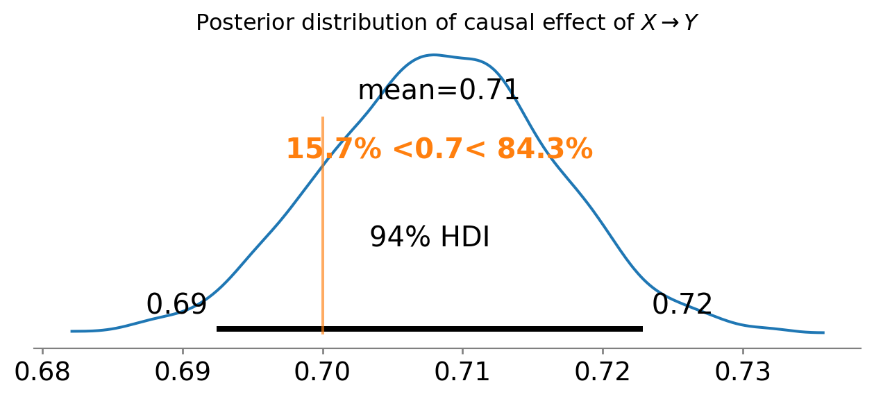
Neat! We have recovered the true causal effect of \(X \rightarrow Y\), but this time we didn’t have to think about the good and bad controls. We just specified the DAG and let Bayes do the rest.
Summary
What have we learned here? We have possibly learnt that we’ve been doing science wrong all this time. You really cannot just throw all your variables into a regression and hope for the best. You need to think about the causal relationships between your variables and then include the good controls. If you include bad controls, then you will get the wrong answer and fool yourself and publish stuff that is wrong.
However, there is a message of hope. If you learn about causal inference, you can do better science. You can get the right answer and publish stuff that is less wrong. So the main question here is how to distinguish the good from the bad controls. That will be the topic of another post.
However, if you are lazy and don’t want to do that, there is another way! You can use Bayesian Structural Causal Modeling. You can specify the DAG (which takes a little more typing) and let the computer do the rest. This is a very powerful approach and one that I am very excited about. I hope you are too.
That said, the overall take-home message of this blogpost is that if you have not started on the causal journey then you should be scared shitless.
If you are interested in this approach of learning about causal inference through simulation, then check out the paper “Why we should teach causal inference: Examples in linear regression with simulated data” (Lübke et al. 2020). And you can follow me on LinkedIn to get notified of future posts.
References
Bulbulia, Joseph, Uffe Schjoedt, John H. Shaver, Richard Sosis, and Wesley J. Wildman. 2021. “Causal Inference in Regression: Advice to Authors.” Religion, Brain & Behavior 11 (4): 353–60. https://doi.org/10.1080/2153599X.2021.2001259.
Capretto, Tomás, Camen Piho, Ravin Kumar, Jacob Westfall, Tal Yarkoni, and Osvaldo A Martin. 2022. “Bambi: A Simple Interface for Fitting Bayesian Linear Models in Python.” Journal of Statistical Software 103 (15): 1–29. https://doi.org/10.18637/jss.v103.i15.
Kumar, Ravin, Colin Carroll, Ari Hartikainen, and Osvaldo Martin. 2019. “ArviZ a Unified Library for Exploratory Analysis of Bayesian Models in Python.” Journal of Open Source Software 4 (33): 1143. https://doi.org/10.21105/joss.01143.
Lübke, Karsten, Matthias Gehrke, Jörg Horst, and Gero Szepannek. 2020. “Why We Should Teach Causal Inference: Examples in Linear Regression with Simulated Data.” Journal of Statistics Education 28 (2): 133–39.
McElreath, Richard. 2020. Statistical Rethinking: A Bayesian Course with Examples in r and Stan. CRC press.
Molak, Aleksander. 2023. Causal Inference and Discovery in Python. Packt Publishing.
Wiecki, Thomas, John Salvatier, Ricardo Vieira, et al. 2023. Pymc-Devs/Pymc: V5.6.1. V. v5.6.1. Zenodo, released July. https://doi.org/10.5281/zenodo.8146216.
Wilkinson, GN, and CE Rogers. 1973. “Symbolic Description of Factorial Models for Analysis of Variance.” Journal of the Royal Statistical Society Series C: Applied Statistics 22 (3): 392–99.
Footnotes
If you are a Bayesian then you will be used to interpreting these kinds of posterior distribution plots. For our present purposes we can just ask whether the credible interval of our posterior distribution is anywhere close to the true value.↩︎