Imagine an online shop deciding whether to spend more money showing ads to people who have already visited its website. That practice is often called retargeting (also called remarketing): after someone visits your site, you show them follow-up ads on other websites/apps to try to bring them back.
The team compares two statistical models trained on past campaign data. In simple terms, both models use information about users (for example past site visits, ad exposures, and engagement signals) to predict an outcome such as whether a user purchases, or how much they spend.
Here is the conflict. Model A has slightly worse fit, but it implies the ads do create meaningful extra purchases, which is broadly in line with the team’s expectation that these ads are doing something useful. Model B has better goodness of fit, but it implies the ads add little or no extra value.
So which model should the team trust: the one that fits the historical data better, or the one that seems more plausible for the intervention decision they actually need to make?
Why does this matter? Because if the team trusts the better-fit model for a causal decision, they may conclude “retargeting is not doing much” and cut a campaign that is actually helping.
That is the core mistake this post is about. In causal-first work, the question is not:
❌ Which model best predicts purchases under the current ad-targeting system?
It is:
✅ Which model best estimates what will happen if we change the ad-targeting system?
This post is about that difference, and I will explain each step in plain language as we go.
The key reason this matters is that models here are being used to inform decisions, and decisions are interventions. Prediction models learn how variables co-vary under the current system, but an intervention changes that system (for example by changing who gets exposed to ads) (Pearl 2009). Once the assignment mechanism changes, even strong out-of-sample predictive performance under the old system is not enough; we need a model that is useful for the interventional question, which is exactly the observational-versus-interventional distribution distinction highlighted in the PyMC example by Vincent (2023). This is a causal-decision version of a broader point emphasized in statistical modeling: predictive performance and explanatory/structural adequacy are different objectives (Breiman 2001; Shmueli 2010).
This post was inspired by Orduz’s collider example showing that higher Bayesian \(R^2\) can coincide with worse causal effect estimation (Orduz 2026). The specific contribution here is to make that lesson operational for model selection in a decision setting: define the causal estimand first, classify candidate features by causal role (proxy, mediator, collider-like bad control), and compare models on both observational fit and the intervention quantity that drives the decision.
Our running example: retargeting and purchases
To make the rest of the post concrete, I will use one running example: an online shop deciding whether retargeting ads cause extra purchases. The core causal question is “What is the causal effect of retargeting exposure on purchases?” At the highest level, this is the relationship we care about:
The complication is that real systems contain many other variables (such as browsing behavior, engagement signals, and targeting rules). Adding those variables to a model can improve predictive fit, but some of them can also bias the causal estimate if they are used in the wrong way.
That is the main tension we will unpack in the next sections: a model can become better at predicting observed data while becoming worse for estimating the causal effect we actually care about.
Roadmap for the rest of the post: first I will define the causal target and show the baseline confounding problem, then I will show two common bad-control mistakes (mediator and collider), and finally I will compare two regression strategies in one simulation to show how fit and causal usefulness can diverge.
Before we look at examples of bad controls, we need to make the baseline causal problem explicit: confounding.
Causal complication: confounding
Suppose we want to estimate the causal effect of showing follow-up ads (retargeting) on purchases. The core problem in this example is confounding: Intent is a confounding variable because it affects both who gets shown ads and who purchases.
That is a problem for causal estimation because a simple comparison of users who saw the ad vs users who did not will mix together:
- the effect of the ad itself, and
- pre-existing differences in how likely people were to buy.
In this example, that pre-existing difference is Intent (how ready someone already was to buy). The Directed Acyclic Graph (DAG) below makes that problem visible.
PriorSiteVisits is an observed proxy for intent and may help adjustment by partially accounting for pre-treatment differences in intent. But it does not change the estimand (the target quantity being estimated): we still want the causal effect of retargeting exposure on purchase.
The quantity we want is still the causal impact of retargeting exposure on purchases. PriorSiteVisits is included to show an important practical point: we often cannot observe intent directly, but we may observe proxies (such as browsing activity) that contain some information about it. Those proxies can sometimes help us adjust for confounding. In the worked example below, this proxy is represented by prior_site_visits, which is measured before retargeting exposure is assigned (so it is pre-treatment, not a mediator). These proxies do not change the target question.
Before we look at two failure-mode DAGs, here is the core distinction in one table. The point is not just “prediction vs causality” in the abstract; it is which target is useful for a decision that changes how the system assigns treatment.
| Goal | Typical target | Useful features | Failure mode |
|---|---|---|---|
| Prediction | “Who will buy?” | Any stable predictive signal | Mistakes correlation for lever |
| Causal decision | “What changes if we show the ad?” (extra purchases caused by the ad; often called uplift) | Causally justified adjustment set | Bias from colliders / mediators / leakage |
Fit metrics are still useful diagnostics. They are just not the causal objective (Shmueli 2010; Breiman 2001).
DAG walkthrough: two ways added variables can hurt causal estimation
Adding variables can improve predictive fit while making the causal estimate worse for the estimand we care about. When model outputs drive interventions, these are not just estimation mistakes; they become decision mistakes. The next two DAGs show two common ways that happens:
- Figure 3: a highly predictive variable is post-treatment (mediator)
- Figure 4: a highly predictive variable is a collider (bad control)
Here, “conditioning on” or “controlling for” means including a variable in the regression model as a predictor (or otherwise holding it fixed during estimation). I start with the broader post-treatment/mediator mistake, then return to the collider pattern. For a concise taxonomy of good and bad controls, see Cinelli et al. (2022).
A. Conditioning on a mediator
There is a common mistake that often looks sensible from a prediction perspective: controlling for variables that happen after the treatment.
Teams often include downstream engagement features because they are close to the outcome and improve prediction. But if your goal is the total effect of the ad, those variables can remove part of the very effect you are trying to measure.
In this DAG, SiteEngagement sits on the pathway from exposure to purchase. That makes it a mediator (a variable through which some of the treatment effect flows).
If your estimand (the quantity you want to estimate) is the total effect of retargeting upon purchase behaviour, controlling for downstream engagement is usually the wrong move. It often improves predictive fit because engagement is close to purchase, but it mechanically removes part of the effect you are trying to estimate.
B. Conditioning on a collider
Now consider a second bad-control pattern: a highly predictive variable that is a collider.
To make the timing explicit, think of PostWindowEngagementScore as an intentionally post-window engagement summary (for example, a downstream CRM/analytics feature aggregated after the campaign and purchase window closes). It can be highly predictive and improve fit metrics, but that is exactly why it is a useful teaching example here: “useful for prediction” does not automatically mean “safe to condition on” for causal estimation. This is different from ordinary pre-purchase engagement features.
This is the same structural collider logic as Orduz’s inquiries example (Orduz 2026), translated into the retargeting setting.
In this DAG, PostWindowEngagementScore is caused by both exposure and purchase. That makes it a collider. Conditioning on a collider can create a spurious path between exposure and purchase, which biases the causal estimate.
So PostWindowEngagementScore can be extremely predictive of purchase and still be the wrong variable to adjust for. This is the specific mechanism behind “fit improves, decision gets worse.”
The worked example in the next section makes this concrete by using one shared data-generating process and comparing two model-building strategies:
- one model that is aligned to the causal target and adjustment set, and
- one model that adds extra predictive features that improve fit but damage the estimated causal effect.
Two regression models: better fit versus better causal decisions
Below is a lightweight simulated example designed for teaching. The aim is not to mimic every detail of a real ad platform. It is to make the causal roles of variables easy to see. The simulated story follows the DAG logic above:
- latent
intent(unobserved “how ready someone is to buy”) affects both exposure and purchase prior_site_visitsis an observed proxy for that intentsite_engagementhappens after exposure (a mediator)post_window_engagement_scoreis a collider-like bad control (intentionally post-window for teaching)
prior_site_visits is a pre-treatment proxy for latent intent, while site_engagement (mediator) and post_window_engagement_score (collider-like, intentionally measured after the campaign window) should not be conditioned on when estimating the total effect of retargeting exposure on purchase value.
We generate simulated data from this DAG to obtain our historical data. The first few rows look like this:
Code
def sigmoid(x):
    return 1 / (1 + np.exp(-x))

N = 4000

# Pre-treatment variables
intent = rng.normal(0, 1, N)                     # latent
prior_site_visits = 0.9 * intent + rng.normal(0, 0.8, N)  # observed proxy

# Treatment assignment (retargeting exposure) depends on intent + visit
exposure_p = sigmoid(-0.2 + 0.9 * intent + 0.6 * prior_site_visits)
retargeting_exposure = rng.binomial(1, exposure_p, N)

# Noise terms for DGP (stored so we can compute truth under intervention)
eps_engagement = rng.normal(0, 0.9, N)
eps_purchase = rng.normal(0, 1.0, N)
eps_clicks = rng.normal(0, 0.8, N)

truth = {
    "beta_exposure_direct": 0.8,       # direct effect on purchase value
    "beta_engagement_from_x": 1.1,     # exposure -> engagement
    "beta_purchase_from_eng": 0.9,     # engagement -> purchase
}

def generate_site_engagement(x, intent, noise):
    return 0.5 * intent + truth["beta_engagement_from_x"] * x + noise

def generate_purchase(x, intent, prior_site_visits, site_engagement, noise):
    return (
        truth["beta_exposure_direct"] * x
        + 0.9 * intent
        + 0.4 * prior_site_visits
        + truth["beta_purchase_from_eng"] * site_engagement
        + noise
    )

site_engagement = generate_site_engagement(retargeting_exposure, intent, eps_engagement)
purchase_value = generate_purchase(
    retargeting_exposure, intent, prior_site_visits, site_engagement, eps_purchase
)

# Collider-like "bad control" for teaching: intentionally post-window, caused by exposure and purchase
post_window_engagement_score = 0.7 * retargeting_exposure + 0.6 * purchase_value + eps_clicks

df = pd.DataFrame(
    {
        "prior_site_visits": prior_site_visits,
        "retargeting_exposure": retargeting_exposure,
        "site_engagement": site_engagement,
        "post_window_engagement_score": post_window_engagement_score,
        "purchase_value": purchase_value,
    }
)

df.head()| prior_site_visits | retargeting_exposure | site_engagement | post_window_engagement_score | purchase_value | |
|---|---|---|---|---|---|
| 0 | -0.226015 | 1 | 1.434008 | 3.405016 | 1.975659 |
| 1 | 0.902433 | 1 | 1.733130 | 2.370920 | 4.525204 |
| 2 | 1.584380 | 1 | 1.981409 | 3.003509 | 4.435321 |
| 3 | 0.314106 | 0 | -0.895695 | -0.604775 | -2.749173 |
| 4 | 1.607601 | 1 | 0.712520 | 3.209975 | 3.378986 |
The main causal quantity we care about in this example is the ATE (average treatment effect). Here, the treatment is retargeting_exposure (shown ad vs not shown ad) and the outcome is purchase_value. In words, the ATE is the average change in purchase value if everyone in the population were shown the ad, compared with if no one were shown the ad.
\[ \text{ATE} = \mathbb{E}[Y(1) - Y(0)] \]
where \(Y(1)\) is the purchase value a person would have if shown the ad, and \(Y(0)\) is the purchase value that same person would have if not shown the ad.
NotePotential outcomes and the fundamental problem of causal inference (short version)
The notation \(Y(1)\) and \(Y(0)\) comes from the potential outcomes framework (Holland 1986). For each person, we can imagine two possible outcomes:
- purchase value if they are shown the ad, \(Y(1)\),
- purchase value if they are not shown the ad, \(Y(0)\).
The problem is that we never observe both for the same person at the same time. We only observe one of them, depending on what actually happened. This is the fundamental problem of causal inference (Holland 1986).
That is why causal inference needs assumptions and modeling: we use observed data (plus a causal model/DAG) to estimate the missing counterfactual outcomes well enough to answer the intervention question. In other words, the decision depends on outcomes we do not directly observe, so “fit to observed outcomes” is not by itself the right target.
Model 1: prediction-focused
This model uses variables that are very informative for prediction, including post-treatment engagement and a collider-like post-window engagement summary.
predictive_formula = "purchase_value ~ retargeting_exposure + prior_site_visits + site_engagement + post_window_engagement_score"
model_predictive = bmb.Model(predictive_formula, data=df)
idata_predictive = model_predictive.fit(draws=1000, tune=1000, random_seed=seed)
This is exactly the kind of model that can look excellent on fit metrics because it includes variables that are close to the outcome.
Model 2: causal-first
For the causal model, we want the total effect of retargeting_exposure on purchase_value, so we need to be explicit about what we condition on in Figure 5.
Adjustment-set logic (concise version):
- We want the total causal effect of
retargeting_exposureonpurchase_value. Intentis a confounder, but it is unobserved.prior_site_visitsis a pre-treatment proxy for intent, so we include it.site_engagementis a mediator (post-treatment), so conditioning on it would block part of the total effect.post_window_engagement_scoreis collider-like in this setup, so conditioning on it can introduce bias.
So the causal-first model conditions on prior_site_visits but not on site_engagement or post_window_engagement_score.
causal_formula = "purchase_value ~ retargeting_exposure + prior_site_visits"
model_causal = bmb.Model(causal_formula, data=df)
idata_causal = model_causal.fit(draws=1000, tune=1000, random_seed=seed)
Compare the models
We’ll take the fitted models and use them to estimate the ATE (the causal quantity we care about) using G-computation. Then we’ll compare the ATE estimates and their uncertainty, along with the in-sample fit metrics. We will evaluate each model twice: once on observational fit to the observed outcomes, and once on the causal estimand (ATE). For the fit comparison, I use an in-sample posterior-mean predictive R^2 computed from the posterior mean of mu (not Bayesian R^2); the causal lesson here does not depend on the exact fit metric.
Code
# Truth-level ATE via intervention on exposure, averaging over same units/noise
eng_1 = generate_site_engagement(np.ones(N), intent, eps_engagement)
eng_0 = generate_site_engagement(np.zeros(N), intent, eps_engagement)
y_1 = generate_purchase(np.ones(N), intent, prior_site_visits, eng_1, eps_purchase)
y_0 = generate_purchase(np.zeros(N), intent, prior_site_visits, eng_0, eps_purchase)
truth_ate = np.mean(y_1 - y_0)

def posterior_mean_r2(model, idata, data, outcome_col):
    # In-sample predictive R^2 from posterior-mean mu (not Bayesian R^2)
    model.predict(idata, data=data, inplace=True)
    mu_mean = idata.posterior["mu"].mean(dim=("chain", "draw")).values
    y = data[outcome_col].to_numpy()
    ss_res = np.sum((y - mu_mean) ** 2)
    ss_tot = np.sum((y - y.mean()) ** 2)
    return 1 - ss_res / ss_tot

def gcomp_ate(model, idata, data, treatment_col, high=1, low=0):
    data_hi = data.copy()
    data_hi[treatment_col] = high
    model.predict(idata, data=data_hi, inplace=True)
    mu_hi = idata.posterior["mu"].copy(deep=True)

    data_lo = data.copy()
    data_lo[treatment_col] = low
    model.predict(idata, data=data_lo, inplace=True)
    mu_lo = idata.posterior["mu"].copy(deep=True)

    ate = (mu_hi - mu_lo).mean(dim="__obs__")
    return ate

ate_causal = gcomp_ate(model_causal, idata_causal, df, "retargeting_exposure")
ate_predictive = gcomp_ate(model_predictive, idata_predictive, df, "retargeting_exposure")

r2_causal = posterior_mean_r2(model_causal, idata_causal, df, "purchase_value")
r2_prediction = posterior_mean_r2(model_predictive, idata_predictive, df, "purchase_value")
NoteHow we estimate the ATE here (G-computation)
We estimate the ATE using G-computation (also called standardization):
- Fit a regression model.
- Predict outcomes if everyone is set to
retargeting_exposure = 1(shown ads). - Predict outcomes if everyone is set to
retargeting_exposure = 0(not shown ads). - Average the difference.
G-computation identifies a causal ATE only under assumptions (including no unmeasured confounding after adjustment, positivity, and an adequate outcome model), and in this simulation we intentionally adjust with a proxy so some residual bias can remain. This turns the fitted regression model into an estimate of the causal quantity defined above by explicitly comparing predicted outcomes under two different hypothetical treatment assignments. That is why it is aligned to the decision question (what happens if we change exposure?) rather than only to observational goodness of fit.
Now let’s plot the results.
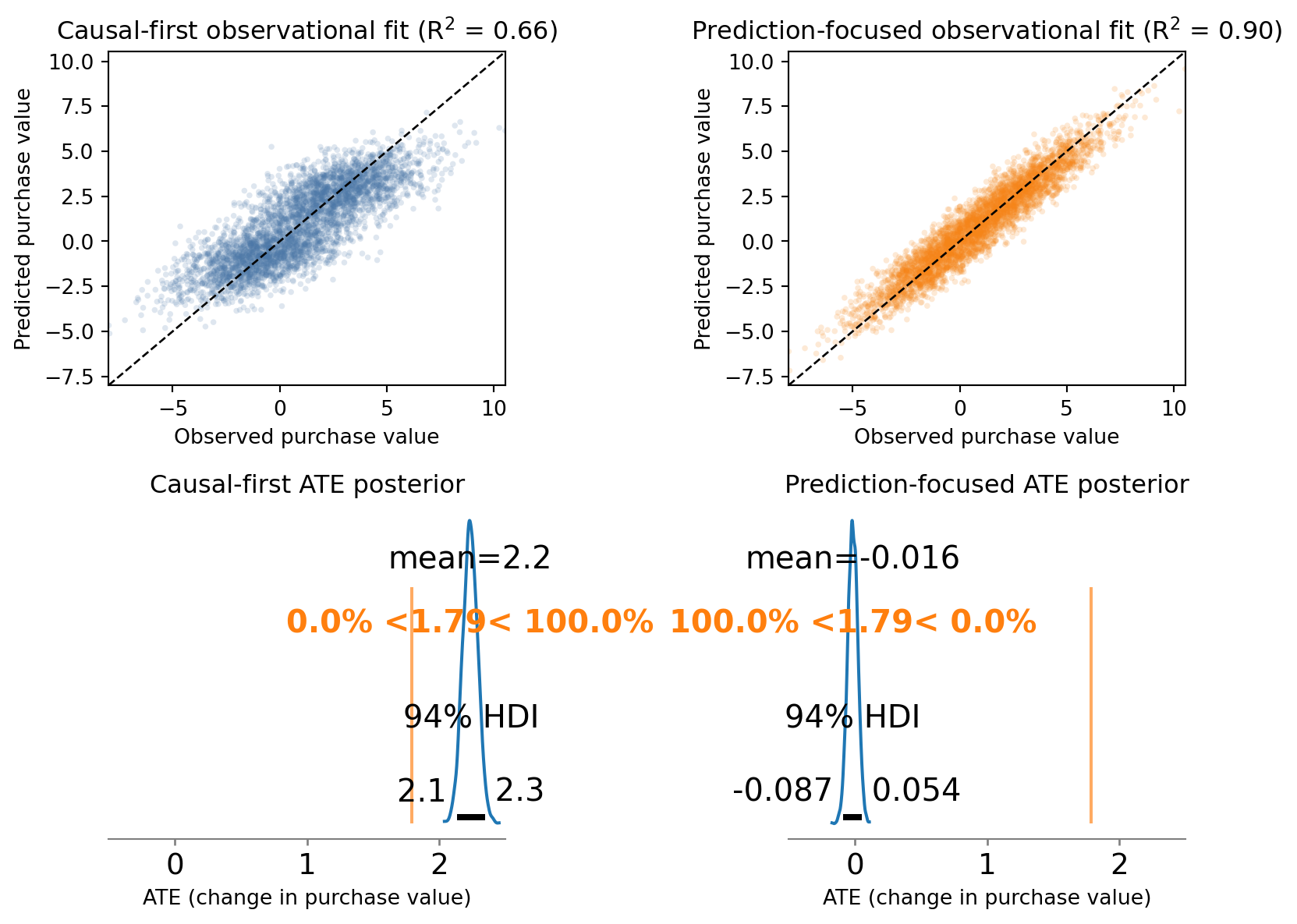
Figure 6 shows the main point of the post in miniature: the prediction-focused model looks much better on observational fit (top row) but is much worse for the causal quantity we care about (bottom row).
What did we learn?
The important extension for decision-making is what happens next. If a team trusted the prediction-focused model, it would conclude that retargeting has little or no causal impact on purchases and may recommend cutting a campaign that is actually useful. The causal-first model is not perfect, but it is much closer to the true intervention effect, so it points toward the better decision.
Even if the prediction-focused model also won on holdout predictive fit (note tested here), that would not fix this problem. The decision changes the treatment assignment mechanism, so the relevant target is the interventional distribution, not just predictive performance under the observational one (that is, under the same assignment policy) (Vincent 2023).
One subtle but important point is that the causal-first model may still miss the true ATE by a noticeable amount. That is not a contradiction. In this simulation, the true confounder (Intent) is unobserved, and we adjust using prior_site_visits, which is only a proxy. The proxy reduces confounding bias, but it does not eliminate it completely, so some residual bias can remain.
The exact numbers will vary with simulation choices, but the pattern is the point:
- the prediction-focused model usually achieves better fit
- its causal ATE estimate is often worse because it controls for variables that should not be used when estimating the total effect
- the causal-first model can still miss the truth if key confounders are unobserved and only partially captured by proxies
So the “better” model depends on what “better” means:
- better forecasting of observed outcomes
- or better estimation of the effect of an intervention
Those are often related, but they are not the same objective.
The model-selection lesson is not “prefer worse goodness of fit” for its own sake. The lesson is that maximizing goodness of fit as the primary objective is the wrong criterion when the model is being used to support intervention decisions.
Summary
The practical message is not “ignore prediction” and it is not “anti-ML.” It is to separate two jobs that are often collapsed into one:
- forecasting what happens under the current assignment system
- estimating what would change under an intervention
In the retargeting example, that separation forced three useful modeling decisions:
- define the causal target first (the total effect of retargeting on purchases)
- classify variables by causal role (proxy, collider, mediator) rather than predictive strength alone
- evaluate the model on the causal quantity and decision relevance, not just goodness of fit
The key reason is the same one introduced at the start of the post: decisions are interventions, and interventions change the system you are modeling. A model that performs well under the observational distribution can still fail under the interventional distribution if it learns the wrong structure for the decision problem (Vincent 2023).
So if your goal is business decisions, budgeting, targeting, or policy changes, the call to action is simple: do not treat predictive power as the primary objective. Start with the causal question, build the model around the intervention and estimand, and use goodness of fit as a diagnostic rather than the goal.
The worked example also shows a more realistic point: even a causally motivated model can remain biased when important confounders are unobserved and only imperfectly proxied. Causal-first modeling does not guarantee perfect recovery, but it does give you a better chance of making the right decision for the right reason.
References
Breiman, Leo. 2001. “Statistical Modeling: The Two Cultures.” Statistical Science 16 (3): 199–231. https://doi.org/10.1214/ss/1009213726.
Cinelli, Carlos, Andrew Forney, and Judea Pearl. 2022. “A Crash Course in Good and Bad Controls.” Sociological Methods & Research, ahead of print. https://doi.org/10.1177/00491241221099552.
Holland, Paul W. 1986. “Statistics and Causal Inference.” Journal of the American Statistical Association 81 (396): 945–60. https://doi.org/10.1080/01621459.1986.10478354.
Orduz, Juan Camilo. 2026. In-Sample R^2 Is Not a Good Metric for Decision Making. https://juanitorduz.github.io/no_r2/.
Pearl, Judea. 2009. Causality: Models, Reasoning, and Inference. 2nd ed. Cambridge University Press.
Shmueli, Galit. 2010. “To Explain or to Predict?” Statistical Science 25 (3): 289–310. https://doi.org/10.1214/10-STS330.
Vincent, Benjamin T. 2023. “Interventional Distributions and Graph Mutation with the Do-Operator.” In PyMC Examples, edited by PyMC Team. https://doi.org/10.5281/zenodo.5654871.