Bayesian models + grammar of graphics + Python = ❤️

python
bayes
data-viz
Author

Benjamin Vincent

Published

April 24, 2025

Why another plotting post?

Bayesian modelling in Python is pretty solid: We’ve got PyMC for model building and inference, ArviZ covers diagnostics and plotting, and we’ve got helpful pacakges like Bambi as a layer on top of PyMC to make linear modelling more convenient.

However, one of the pain points I often encounter is on the plotting side of things. Even for relatively simple models, if you want to get some nice data viz out to deliver some sweet insights to stakeholders, or even just sanity check the results, it can be a bit of a pain. At the moment you have to be pretty familiar with the internals of the arviz.InferenceData object and do a whole bunch of wrangling to get what you need in order to plot it. This often involves imperative style telling the computer what to do (slice this dimension, aggregate that dimension, loop over this group etc.).

So I’ve been left wondering:

Can we make the plotting of Bayesian models in Python more declarative?

This post is a quick exploration of that idea. I don’t have a full solution, but I do have a proof of concept that shows how we can get a grammar-of-graphics approach to plotting Bayesian models in Python.

Setting up the data and modelling that we’ll plot

First, we need to generate some data, build a PyMC model, and sample from it. We’ll also generate a grid of points to evaluate the posterior predictive distribution on. At the end of this we’ll have a bunch of MCMC samples from the posterior distribution of the model. This will be stored in an arviz.InferenceData object. We’ll hide all these steps because they are not the focus of this post. But you can un-collapse the code block if you want to see the details.

Code
import arviz as az
import matplotlib.pyplot as plt
import pandas as pd
import numpy as np
import pymc as pm
import seaborn as sns
from plotnine import (
    ggplot,
    aes,
    stat_summary,
    facet_wrap,
    theme_classic,
    labs,
    geom_density,
    geom_point,
)

plt.rcParams["figure.figsize"] = [8, 5]
%config InlineBackend.figure_format = 'retina'

RANDOM_SEED = 42
rng = np.random.default_rng(RANDOM_SEED)

# generate data ------------------------------------------------------------------------
n_groups = 4
group_size = [2, 4, 6, 8]

# Group-specific parameters
slopes = rng.normal(1, 0.2, size=n_groups)
intercepts = rng.normal(0, 1, size=n_groups)

# Generate data
data = []
for i in range(n_groups):
    n = group_size[i]
    x_vals = np.sort(rng.uniform(0, 20, size=n))
    noise = rng.normal(0, 1, size=n)
    y_vals = slopes[i] * x_vals + intercepts[i] + noise
    group_labels = np.full(n, i)
    data.append(pd.DataFrame({"x": x_vals, "y": y_vals, "group": group_labels}))

# Combine all groups into a single DataFrame
df = pd.concat(data, ignore_index=True)
df["group"] = df["group"].astype("category")

# Build a PyMC model -------------------------------------------------------------------
prior_mean = 0
prior_std = 1

x_data = df.x.values
y_data = df.y.values

coords = {"groups": df["group"].cat.categories, "obs_ind": df.index}

with pm.Model(coords=coords) as _m:
    x = pm.Data("x", x_data, dims="obs_ind")
    y = pm.Data("y", y_data, dims="obs_ind")
    group = pm.Data("group", df["group"].cat.codes.values, dims="obs_ind")
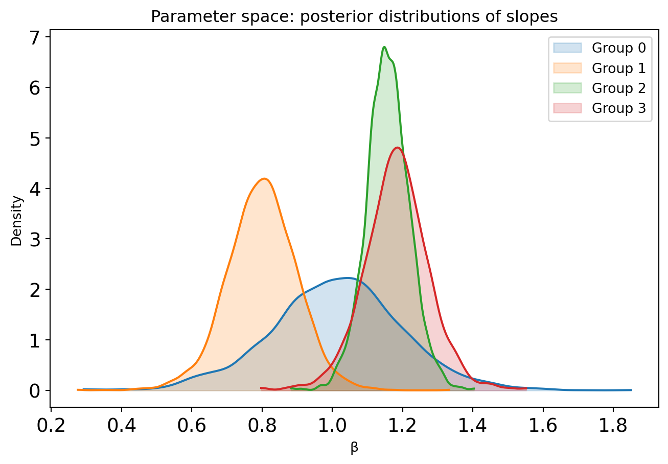
    # priors
    intercept = pm.Normal("intercept", mu=0, sigma=10, dims=["groups"])
    beta = pm.Normal("beta", mu=prior_mean, sigma=prior_std, dims=["groups"])
    sigma = pm.HalfNormal("sigma", sigma=5)
    # likelihood
    mu = pm.Deterministic("mu", intercept[group] + beta[group] * x, dims="obs_ind")
    pm.Normal("obs", mu=mu, sigma=sigma, observed=y, dims="obs_ind")
    # sample
    idata = pm.sample()

# Generate a grid of points to evaluate on ---------------------------------------------
n_interp_points = 20
xi = np.concatenate(
    [
        np.linspace(group[1].x.min(), group[1].x.max(), n_interp_points)
        for group in df.groupby("group")
    ]
)
g = np.concatenate([[i] * n_interp_points for i in range(n_groups)]).astype(int)
predict_at = {"x": xi, "group": g, "y": np.zeros_like(xi)}

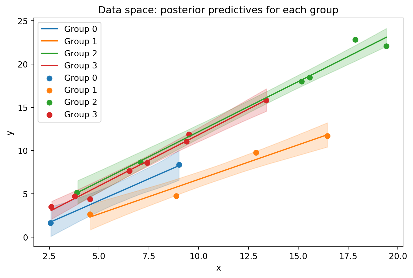
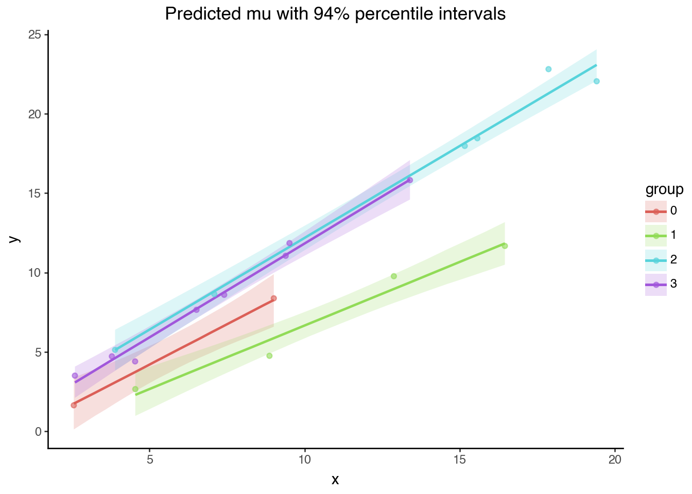
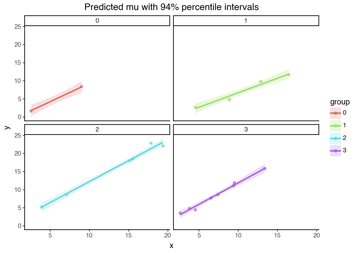
# Posterior prediction on the grid of points -------------------------------------------
coords = {"groups": predict_at["group"], "obs_ind": np.arange(len(xi))}

with _m:
    pm.set_data(predict_at, coords=coords)
    idata.extend(
        pm.sample_posterior_predictive(
            idata,
            var_names=["mu", "y"],
            random_seed=rng,
            progressbar=False,
            predictions=True,
        )
    )

Ok, so after that we now have the following arviz.InferenceData object. You can click on the dropdowns to get more information about the contents of the object. In short, it contains MCMC samples and data.s

arviz.InferenceData
    • <xarray.Dataset> Size: 936kB
      Dimensions:    (chain: 4, draw: 1000, groups: 4, obs_ind: 20)
      Coordinates:
        * chain      (chain) int64 32B 0 1 2 3
        * draw       (draw) int64 8kB 0 1 2 3 4 5 6 7 ... 993 994 995 996 997 998 999
        * groups     (groups) int64 32B 0 1 2 3
        * obs_ind    (obs_ind) int64 160B 0 1 2 3 4 5 6 7 ... 12 13 14 15 16 17 18 19
      Data variables:
          intercept  (chain, draw, groups) float64 128kB -0.4746 -1.427 ... 2.804
          beta       (chain, draw, groups) float64 128kB 0.9442 0.7746 ... 0.9095
          sigma      (chain, draw) float64 32kB 0.7011 0.6883 0.597 ... 1.591 1.37
          mu         (chain, draw, obs_ind) float64 640kB 1.945 8.03 ... 11.46 14.99
      Attributes:
          created_at:                 2025-05-02T14:24:27.321753+00:00
          arviz_version:              0.21.0
          inference_library:          pymc
          inference_library_version:  5.22.0
          sampling_time:              1.5654027462005615
          tuning_steps:               1000

    • <xarray.Dataset> Size: 5MB
      Dimensions:  (chain: 4, draw: 1000, obs_ind: 80)
      Coordinates:
        * chain    (chain) int64 32B 0 1 2 3
        * draw     (draw) int64 8kB 0 1 2 3 4 5 6 7 ... 993 994 995 996 997 998 999
        * obs_ind  (obs_ind) int64 640B 0 1 2 3 4 5 6 7 8 ... 72 73 74 75 76 77 78 79
      Data variables:
          mu       (chain, draw, obs_ind) float64 3MB 1.945 2.265 ... 14.47 14.99
          y        (chain, draw, obs_ind) float64 3MB 0.0 0.0 0.0 0.0 ... 0.0 0.0 0.0
      Attributes:
          created_at:                 2025-05-02T14:24:27.413261+00:00
          arviz_version:              0.21.0
          inference_library:          pymc
          inference_library_version:  5.22.0

    • <xarray.Dataset> Size: 496kB
      Dimensions:                (chain: 4, draw: 1000)
      Coordinates:
        * chain                  (chain) int64 32B 0 1 2 3
        * draw                   (draw) int64 8kB 0 1 2 3 4 5 ... 995 996 997 998 999
      Data variables: (12/17)
          energy_error           (chain, draw) float64 32kB -0.5604 0.2792 ... 0.0619
          reached_max_treedepth  (chain, draw) bool 4kB False False ... False False
          acceptance_rate        (chain, draw) float64 32kB 0.9922 0.8937 ... 0.9854
          diverging              (chain, draw) bool 4kB False False ... False False
          energy                 (chain, draw) float64 32kB 45.97 45.99 ... 53.51
          index_in_trajectory    (chain, draw) int64 32kB 8 -4 1 -10 7 ... 12 4 11 -2
          ...                     ...
          step_size              (chain, draw) float64 32kB 0.2877 0.2877 ... 0.2709
          process_time_diff      (chain, draw) float64 32kB 0.000489 ... 0.000262
          smallest_eigval        (chain, draw) float64 32kB nan nan nan ... nan nan
          perf_counter_start     (chain, draw) float64 32kB 6.765e+05 ... 6.765e+05
          step_size_bar          (chain, draw) float64 32kB 0.2695 0.2695 ... 0.2744
          lp                     (chain, draw) float64 32kB -41.07 -44.0 ... -51.52
      Attributes:
          created_at:                 2025-05-02T14:24:27.332355+00:00
          arviz_version:              0.21.0
          inference_library:          pymc
          inference_library_version:  5.22.0
          sampling_time:              1.5654027462005615
          tuning_steps:               1000

    • <xarray.Dataset> Size: 320B
      Dimensions:  (obs_ind: 20)
      Coordinates:
        * obs_ind  (obs_ind) int64 160B 0 1 2 3 4 5 6 7 8 ... 12 13 14 15 16 17 18 19
      Data variables:
          obs      (obs_ind) float64 160B 1.647 8.383 2.666 ... 11.06 11.86 15.82
      Attributes:
          created_at:                 2025-05-02T14:24:27.335212+00:00
          arviz_version:              0.21.0
          inference_library:          pymc
          inference_library_version:  5.22.0

    • <xarray.Dataset> Size: 400B
      Dimensions:  (obs_ind: 20)
      Coordinates:
        * obs_ind  (obs_ind) int64 160B 0 1 2 3 4 5 6 7 8 ... 12 13 14 15 16 17 18 19
      Data variables:
          x        (obs_ind) float64 160B 2.562 9.008 4.545 8.868 ... 9.391 9.514 13.4
          group    (obs_ind) int32 80B 0 0 1 1 1 1 2 2 2 2 2 2 3 3 3 3 3 3 3 3
      Attributes:
          created_at:                 2025-05-02T14:24:27.335975+00:00
          arviz_version:              0.21.0
          inference_library:          pymc
          inference_library_version:  5.22.0

    • <xarray.Dataset> Size: 2kB
      Dimensions:  (obs_ind: 80)
      Coordinates:
        * obs_ind  (obs_ind) int64 640B 0 1 2 3 4 5 6 7 8 ... 72 73 74 75 76 77 78 79
      Data variables:
          x        (obs_ind) float64 640B 2.562 2.902 3.241 3.58 ... 12.26 12.83 13.4
          group    (obs_ind) int32 320B 0 0 0 0 0 0 0 0 0 0 0 ... 3 3 3 3 3 3 3 3 3 3
      Attributes:
          created_at:                 2025-05-02T14:24:27.414827+00:00
          arviz_version:              0.21.0
          inference_library:          pymc
          inference_library_version:  5.22.0

We can see it contains a number of blocks, some of which are most relevant for our purposes:

  • The posterior block contains MCMC samples from the posterior distribution of the model parameters.
  • The predictions block contains posterior predictive samples for the mu and y variables. The mu variable is the mean of the normal distribution, while y is the observed data.
  • The predictions_constant_data block contains the constant data used in the model to generate the predictions. This is our grid of points where we evaluated the posterior predictive distribution.

Plotting imperatively with arviz

First, we’ll use the amazing (imperative) plotting capabilities of arviz. This is the go-to package to visualize the outputs of Bayesian models in Python - although the package does more than just the visualization side of things.

You can tell that this follows an imperative style because we are doing lots of manual things which don’t actually have anything to do with plotting. For example, we are iterating over the groups, creating masks, looking up subsets of data with those masks, and so on. This is all very low level - it can be fine when you have experience with it, but fundamentally there is a lot of boilerplate and munging of the data, rather than just saying what we want to plot.

fig, ax = plt.subplots()
for group in np.unique(predict_at["group"]):
    group_mask = predict_at["group"] == group
    x_group = predict_at["x"][group_mask]
    y_group = idata.predictions["mu"].isel(obs_ind=group_mask)
    plt.plot(x_group, y_group.mean(dim=["chain", "draw"]), label=f"Group {group}")
    az.plot_hdi(
        x_group,
        y_group,
        hdi_prob=0.95,
        color=sns.color_palette()[group],
        fill_kwargs={"alpha": 0.2},
        ax=ax,
    )
ax.set(title="Data space: posterior predictives for each group", xlabel="x", ylabel="y")

# plot the data
for g in np.unique(df["group"]):
    plt.scatter(
        df["x"][df["group"] == g], df["y"][df["group"] == g], label=f"Group {g}"
    )
plt.legend()

Just for good measure, let’s use the same Bayesian model results and generate a plot of the posterior distributions of the slopes for each group in parameters space. The code snippet below is not very bad at all. However, it still requires a good mental model of the internal structure of the InferenceData object. Though the powerful sel method of xarray is nice.

fig, ax = plt.subplots()
for group in np.unique(idata.predictions_constant_data["group"]):
    az.plot_dist(
        idata["posterior"]["beta"].sel(groups=group),
        label=f"Group {group}",
        color=sns.color_palette()[group],
        fill_kwargs={"alpha": 0.2},
        ax=ax,
    )
ax.set(
    title="Parameter space: posterior distributions of slopes",
    xlabel="β",
    ylabel="Density",
)
[Text(0.5, 1.0, 'Parameter space: posterior distributions of slopes'),
 Text(0.5, 0, 'β'),
 Text(0, 0.5, 'Density')]

Plotting Bayesian models declaratively

The main thing we need to do is to convert the arviz.InferenceData object into a pandas.DataFrame object. More specifically, it needs to be in a tidybayes format.

Step 1: Convert the arviz.InferenceData object to a tidy dataframe

Note that this is the only really novel part of this post - the conversion of the InferenceData object to a tidy dataframe. The rest of the code is just using the plotnine package to plot the data.

Warning

The function below is not very general - it has hard-coded parameter names for example so it won’t work for all models. It would take a bit more work to make it general, but it’s doable!

def make_tidy(idata: az.InferenceData) -> pd.DataFrame:
    """A not very general function to convert an InferenceData object into a tidy
    dataframe."""

    coef_df = (
        idata.posterior[["beta", "intercept"]]
        .to_dataframe()
        .reset_index()
        .rename(columns={"groups": "group"})
    )

    mu_df = idata.predictions["mu"].to_dataframe(name="mu").reset_index()

    const_df = idata.predictions_constant_data.to_dataframe().reset_index()

    mu_df = mu_df.merge(const_df, on="obs_ind", how="left")
    return mu_df.merge(coef_df, on=["chain", "draw", "group"], how="left")


tidy_df = make_tidy(idata)

So let’s use that with our InferenceData object and see what we get out.

chain draw obs_ind mu x group beta intercept
0 0 0 0 1.944707 2.562273 0 0.944191 -0.474568
1 0 0 1 2.265008 2.901507 0 0.944191 -0.474568
2 0 0 2 2.585310 3.240741 0 0.944191 -0.474568
3 0 0 3 2.905611 3.579975 0 0.944191 -0.474568
4 0 0 4 3.225913 3.919209 0 0.944191 -0.474568
... ... ... ... ... ... ... ... ...
319995 3 999 75 12.920041 11.123048 3 0.909456 2.804114
319996 3 999 76 13.436892 11.691356 3 0.909456 2.804114
319997 3 999 77 13.953744 12.259664 3 0.909456 2.804114
319998 3 999 78 14.470595 12.827972 3 0.909456 2.804114
319999 3 999 79 14.987446 13.396280 3 0.909456 2.804114

320000 rows × 8 columns

Well, that’s quite a lot of rows! But the key thing here is that we’ve got both data and parameters into a single tidy dataframe.

Step 2: Plot!

Now we have everything we need to plot the outputs declaratively with plotnine:

p = (
    ggplot(
        tidy_df,
        aes("x", "mu", group="group", color="factor(group)", fill="factor(group)"),
    )
    + stat_summary(
        geom="ribbon",
        fun_ymin=lambda y: np.quantile(y, 0.03),
        fun_ymax=lambda y: np.quantile(y, 0.97),
        alpha=0.20,
        size=0,
    )
    + stat_summary(geom="line", fun_y=np.median, size=1)
    + theme_classic()
    + labs(
        x="x",
        y="y",
        fill="group",
        color="group",
        title=r"Predicted mu with 94% percentile intervals",
    )
    + geom_point(df, aes("x", "y", color="factor(group)"), size=1.6, alpha=0.6)
)
p

So that is certainly not a 1-liner, but it is declarative! Every piece of that code relates to what we want to plot.

One advantage you get from this is that it’s much easier to customize the plot because you are in grammar of graphics territory. For example, we can just add a facet_wrap to completely change the pixels being plotted.

p + facet_wrap('group')

And now let’s see how we can plot the posterior distributions of the slopes for each group in parameters space.

(
    ggplot(tidy_df, aes(x="beta", color="factor(group)"))
    + geom_density(alpha=0.2, size=1)
    + theme_classic()
)

Admittedly, these defaults for plotnine are not great. It is totally possible to customize them, but I’m not doing that here.

Summary

This approach will not necessarily lead to plotting complex graphics in a single line of code, but it does allow you to build up plots in a modular way. This is the main advantage of the grammar of graphics approach - you can build up complex graphics from simple components. And the code you are writing is all about what you want to plot, rather than how to wrangle the data. This is a big difference in terms of mental model and can make it easier to understand what is going on.

Some people may love this, some may be indifferent, some may hate it. Either way, the main point I am making in this blog post is: if you want to to do Bayesian model data viz in a different way, you can do that in Python.

Readers should note that you’ve been able to do this in R for a while now with the ggplot2 and tidybayes packages. It would be interesting to see if this approach is appealing to people. We could even build more geoms and stats or use other grammar of graphics based pagages.