# Showcase
`tidydraws` is tested against synthetic ArviZ objects. This page stress-tests the full pipeline -- PyMC model → ArviZ object → [parameter_draws](../../reference/parameter_draws.md#tidydraws.parameter_draws) / [prediction_draws](../../reference/prediction_draws.md#tidydraws.prediction_draws) / [compare_draws](../../reference/compare_draws.md#tidydraws.compare_draws) → plot -- across eight model archetypes that each exercise a different code path. If this page builds, the data layer survived that shape. If it breaks, you know exactly which archetype is the culprit.
Code
``` python
from pathlib import Path
import sys
import numpy as np
import polars as pl
import tidydraws as td
import lets_plot as lp
import plotnine as p9
for parent in [Path.cwd(), *Path.cwd().parents]:
helper_dir = parent / "docs" / "examples"
if (helper_dir / "_showcase_models.py").exists():
sys.path.insert(0, str(helper_dir))
break
from _showcase_models import (
simple_regression,
varying_intercepts,
varying_slopes,
varying_both,
multiple_regression,
logistic,
simple_regression_1chain,
)
lp.LetsPlot.setup_html()
```
# 1. Simple linear regression
Scalar parameters only -- no group dimensions. Exercises the simplest extraction path.
``` python
dt, obs = simple_regression(seed=2026)
```
Sampling: [alpha, beta, sigma, y]
Initializing NUTS using jitter+adapt_diag...
Multiprocess sampling (2 chains in 2 jobs)
NUTS: [alpha, beta, sigma]
Sampling 2 chains for 400 tune and 400 draw iterations (800 + 800 draws total) took 0 seconds.
We recommend running at least 4 chains for robust computation of convergence diagnostics
Sampling: []
## Use tidydraws
``` python
draws = td.parameter_draws(dt, "alpha", "beta", "sigma")
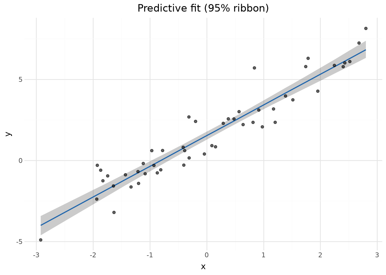
pred = td.prediction_draws(dt, newdata=obs, var_name="mu")
pred_summary = td.point_interval(
pred, "mu", group_by=["obs_ind", "x", "y"], probs=(0.50, 0.80, 0.95)
)
```
Cross-join detected between frame 0 and 1. Broadcasting scalar or differently-dimensioned variable on dims ['chain', 'draw'].
Cross-join detected between frame 1 and 2. Broadcasting scalar or differently-dimensioned variable on dims ['chain', 'draw'].
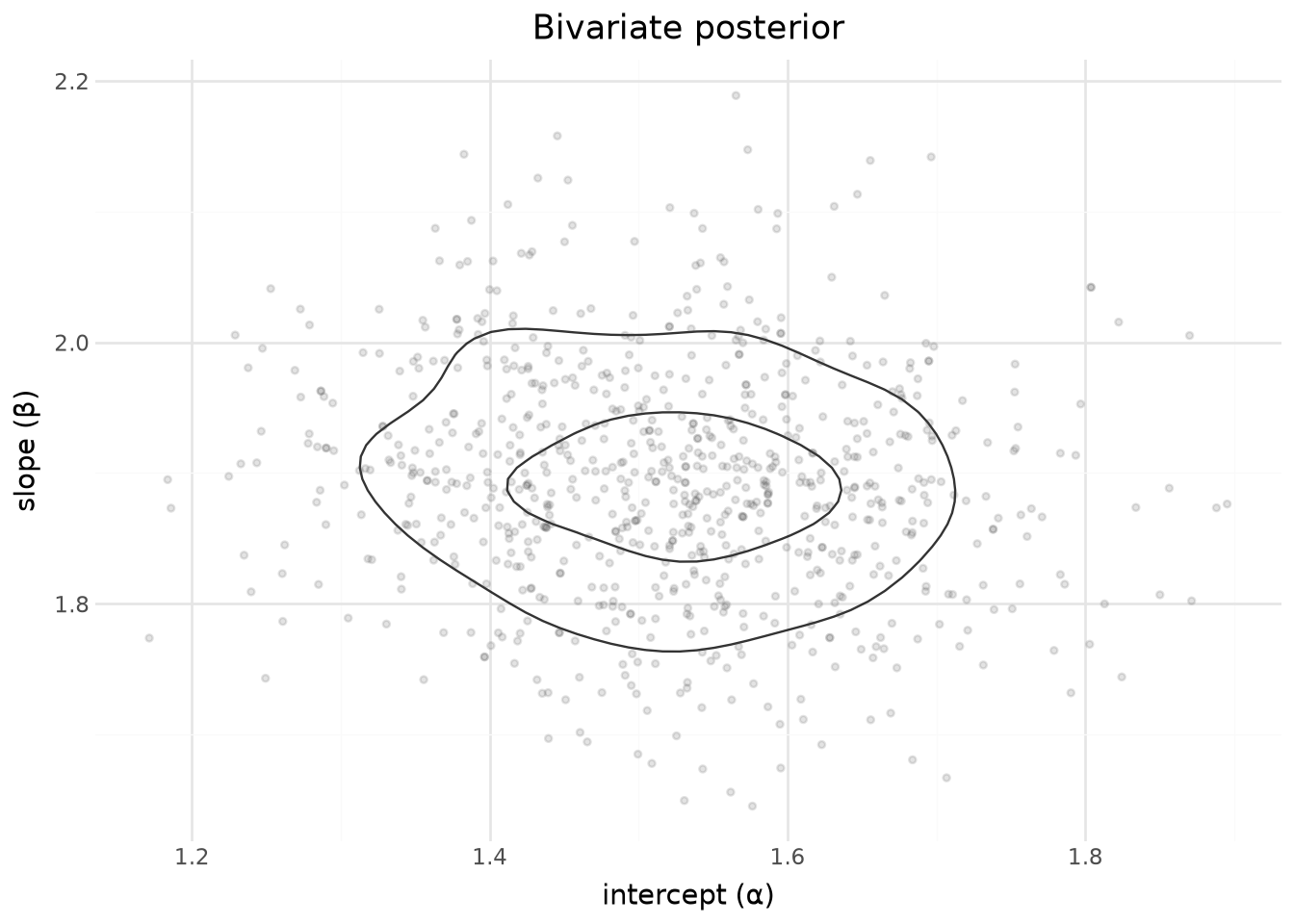
## Bivariate posterior of intercept and slope
`parameter_draws(dt, "alpha", "beta")` returns both columns on the same `chain × draw` index, so a 2D density contour uses them directly.
- lets-plot
- plotnine
``` python
(
lp.ggplot(draws.to_pandas(), lp.aes("alpha", "beta"))
+ lp.geom_density2d(bins=8, alpha=0.8)
+ lp.geom_point(alpha=0.15, size=1.0, color="#444444")
+ lp.labs(x="intercept (α)", y="slope (β)", title="Bivariate posterior")
+ lp.theme_minimal()
)
```
``` python
(
p9.ggplot(draws.to_pandas(), p9.aes("alpha", "beta"))
+ p9.geom_density_2d(alpha=0.8)
+ p9.geom_point(alpha=0.15, size=1.0, color="#444444")
+ p9.labs(x="intercept (α)", y="slope (β)", title="Bivariate posterior")
+ p9.theme_minimal()
)
```
# 2. Varying intercepts
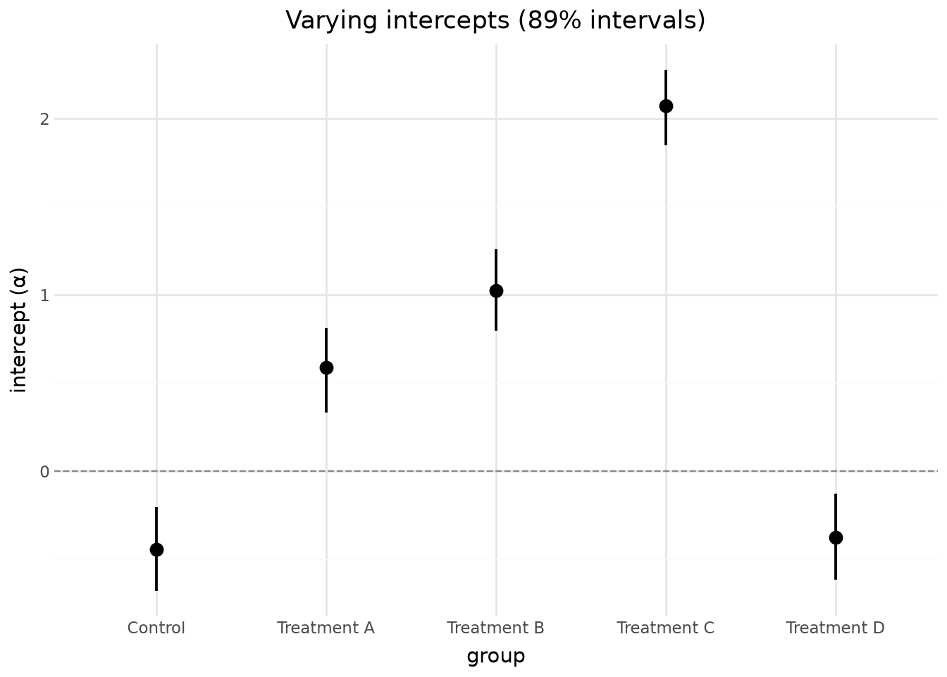
One-dimensional `alpha[group]` with string coordinate labels. Exercises `_group_to_df` with non-numeric coords and tests that forest-plot sorting/filtering works on string dims.
## Use tidydraws
``` python
dt, obs = varying_intercepts(seed=2027)
draws = td.parameter_draws(dt, "alpha")
forest = td.point_interval(draws, "alpha", group_by="group", probs=(0.50, 0.89))
```
Initializing NUTS using jitter+adapt_diag...
Multiprocess sampling (2 chains in 2 jobs)
NUTS: [alpha, beta, sigma]
Sampling 2 chains for 400 tune and 400 draw iterations (800 + 800 draws total) took 1 seconds.
We recommend running at least 4 chains for robust computation of convergence diagnostics
## Forest plot with string labels
- lets-plot
- plotnine
``` python
(
lp.ggplot(forest.to_pandas(), lp.aes("group", "alpha"))
+ lp.geom_pointrange(
lp.aes(ymin="alpha_lower_0.89", ymax="alpha_upper_0.89"), size=0.8
)
+ lp.geom_hline(yintercept=0, linetype="dashed", color="#888888")
+ lp.labs(x="group", y="intercept (α)", title="Varying intercepts (89% intervals)")
+ lp.theme_minimal()
)
```
``` python
(
p9.ggplot(forest.to_pandas(), p9.aes("group", "alpha"))
+ p9.geom_pointrange(
p9.aes(ymin="alpha_lower_0.89", ymax="alpha_upper_0.89"), size=0.8
)
+ p9.geom_hline(yintercept=0, linetype="dashed", color="#888888")
+ p9.labs(x="group", y="intercept (α)", title="Varying intercepts (89% intervals)")
+ p9.theme_minimal()
)
```
# 3. Varying slopes -- cross-dim broadcast
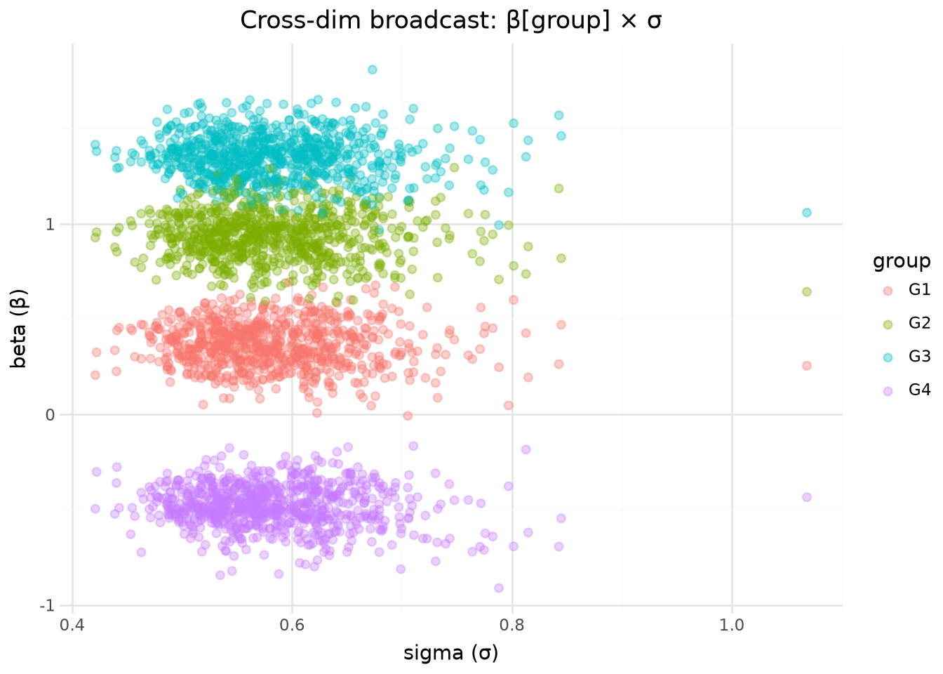
Extracts `beta[group]` (1-d) and scalar `sigma` together. `sigma` is broadcast across all groups -- verifies the cross-dim join doesn't create phantom rows.
``` python
dt, obs = varying_slopes(seed=2028)
```
Sampling: [alpha, beta, sigma]
Initializing NUTS using jitter+adapt_diag...
Multiprocess sampling (2 chains in 2 jobs)
NUTS: [alpha, beta, sigma]
Sampling 2 chains for 400 tune and 400 draw iterations (800 + 800 draws total) took 0 seconds.
We recommend running at least 4 chains for robust computation of convergence diagnostics
The rhat statistic is larger than 1.01 for some parameters. This indicates problems during sampling. See https://arxiv.org/abs/1903.08008 for details
## Use tidydraws
``` python
draws = td.parameter_draws(dt, "beta", "sigma")
```
Cross-join detected between frame 0 and 1. Broadcasting scalar or differently-dimensioned variable on dims ['chain', 'draw'].
## Beta vs sigma scatter
Every group-level beta draw gets the corresponding chain/draw sigma value via broadcast.
- lets-plot
- plotnine
``` python
(
lp.ggplot(draws.to_pandas(), lp.aes("sigma", "beta"))
+ lp.geom_point(lp.aes(color="group"), alpha=0.35, size=2.0)
+ lp.labs(
x="sigma (σ)",
y="beta (β)",
color="group",
title="Cross-dim broadcast: β[group] × σ",
)
+ lp.theme_minimal()
)
```
``` python
(
p9.ggplot(draws.to_pandas(), p9.aes("sigma", "beta"))
+ p9.geom_point(p9.aes(color="group"), alpha=0.35, size=2.0)
+ p9.labs(
x="sigma (σ)",
y="beta (β)",
color="group",
title="Cross-dim broadcast: β[group] × σ",
)
+ p9.theme_minimal()
)
```
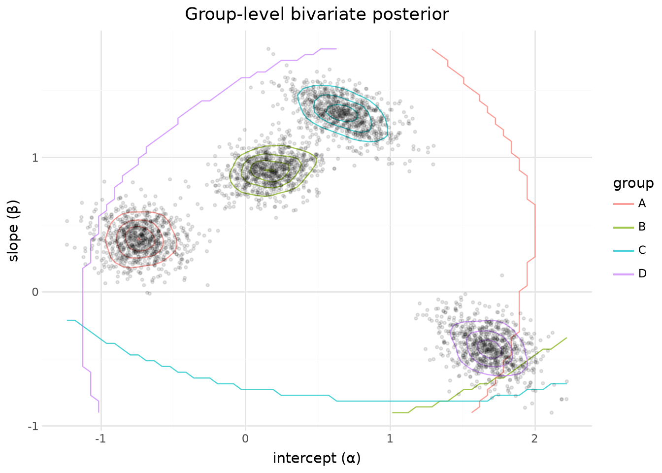
# 4. Bivariate group-level posterior
Two 1-d arrays on the same dimensions: `alpha[group]` and `beta[group]`. [parameter_draws](../../reference/parameter_draws.md#tidydraws.parameter_draws) joins them -- exercises the same-dims multi-variable path.
## Use tidydraws
``` python
dt, obs = varying_both(seed=2029)
draws = td.parameter_draws(dt, "alpha", "beta")
```
Initializing NUTS using jitter+adapt_diag...
Multiprocess sampling (2 chains in 2 jobs)
NUTS: [alpha, beta, sigma]
Sampling 2 chains for 400 tune and 400 draw iterations (800 + 800 draws total) took 1 seconds.
We recommend running at least 4 chains for robust computation of convergence diagnostics
## 2D density by group
- lets-plot
- plotnine
``` python
(
lp.ggplot(draws.to_pandas(), lp.aes("alpha", "beta"))
+ lp.geom_density2d(lp.aes(color="group"), bins=5, alpha=0.7)
+ lp.geom_point(alpha=0.10, size=0.8)
+ lp.labs(
x="intercept (α)",
y="slope (β)",
color="group",
title="Group-level bivariate posterior",
)
+ lp.theme_minimal()
)
```
``` python
(
p9.ggplot(draws.to_pandas(), p9.aes("alpha", "beta"))
+ p9.geom_density_2d(p9.aes(color="group"), alpha=0.7)
+ p9.geom_point(alpha=0.10, size=0.8)
+ p9.labs(
x="intercept (α)",
y="slope (β)",
color="group",
title="Group-level bivariate posterior",
)
+ p9.theme_minimal()
)
```
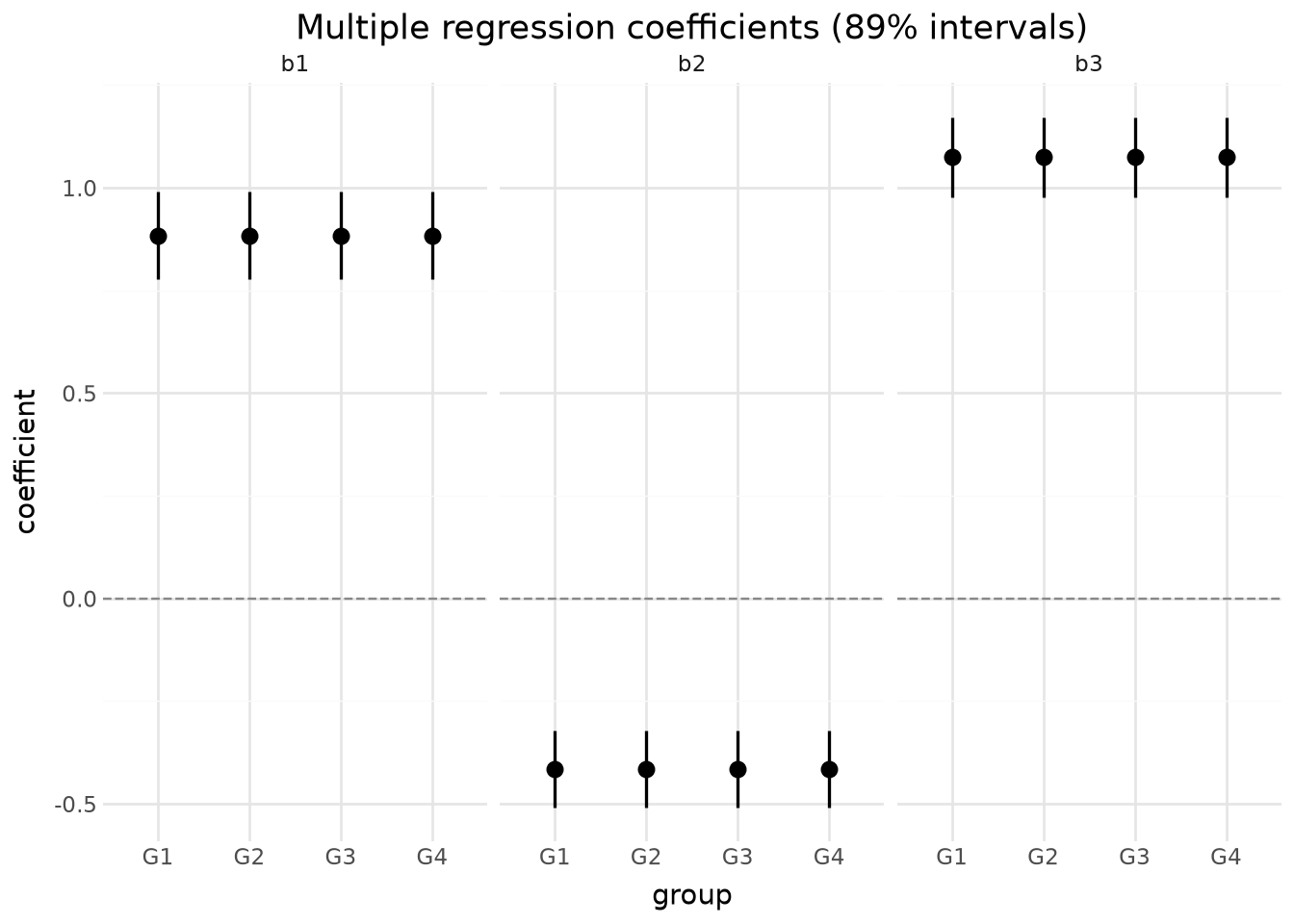
# 5. Multiple regression
Three scalar predictors, varying intercepts per group. [parameter_draws](../../reference/parameter_draws.md#tidydraws.parameter_draws) extracts `b1`, `b2`, `b3`, and `alpha[group]` -- four variables, three of them scalar, one 1-d. Exercises many-variable alignment.
``` python
dt, obs = multiple_regression(seed=2030)
```
Initializing NUTS using jitter+adapt_diag...
Multiprocess sampling (2 chains in 2 jobs)
NUTS: [alpha, b1, b2, b3, sigma]
Sampling 2 chains for 400 tune and 400 draw iterations (800 + 800 draws total) took 1 seconds.
We recommend running at least 4 chains for robust computation of convergence diagnostics
The rhat statistic is larger than 1.01 for some parameters. This indicates problems during sampling. See https://arxiv.org/abs/1903.08008 for details
## Use tidydraws
``` python
draws = td.parameter_draws(dt, "b1", "b2", "b3", "alpha")
coefs = pl.concat([
draws.select(pl.col("group"), pl.col("b1").alias("value")).with_columns(
pl.lit("b1").alias("predictor")
),
draws.select(pl.col("group"), pl.col("b2").alias("value")).with_columns(
pl.lit("b2").alias("predictor")
),
draws.select(pl.col("group"), pl.col("b3").alias("value")).with_columns(
pl.lit("b3").alias("predictor")
),
])
coef_forest = td.point_interval(
coefs, "value", group_by=["predictor", "group"], probs=(0.89,)
)
```
Cross-join detected between frame 0 and 1. Broadcasting scalar or differently-dimensioned variable on dims ['chain', 'draw'].
Cross-join detected between frame 1 and 2. Broadcasting scalar or differently-dimensioned variable on dims ['chain', 'draw'].
Cross-join detected between frame 2 and 3. Broadcasting scalar or differently-dimensioned variable on dims ['chain', 'draw'].
## Faceted coefficient forest
- lets-plot
- plotnine
``` python
(
lp.ggplot(coef_forest.to_pandas(), lp.aes("group", "value"))
+ lp.geom_pointrange(lp.aes(ymin="value_lower", ymax="value_upper"), size=0.7)
+ lp.geom_hline(yintercept=0, linetype="dashed", color="#888888")
+ lp.facet_wrap(facets="predictor", ncol=3)
+ lp.labs(
x="group",
y="coefficient",
title="Multiple regression coefficients (89% intervals)",
)
+ lp.theme_minimal()
)
```
``` python
(
p9.ggplot(coef_forest.to_pandas(), p9.aes("group", "value"))
+ p9.geom_pointrange(p9.aes(ymin="value_lower", ymax="value_upper"), size=0.7)
+ p9.geom_hline(yintercept=0, linetype="dashed", color="#888888")
+ p9.facet_wrap("~predictor", ncol=3)
+ p9.labs(
x="group",
y="coefficient",
title="Multiple regression coefficients (89% intervals)",
)
+ p9.theme_minimal()
)
```
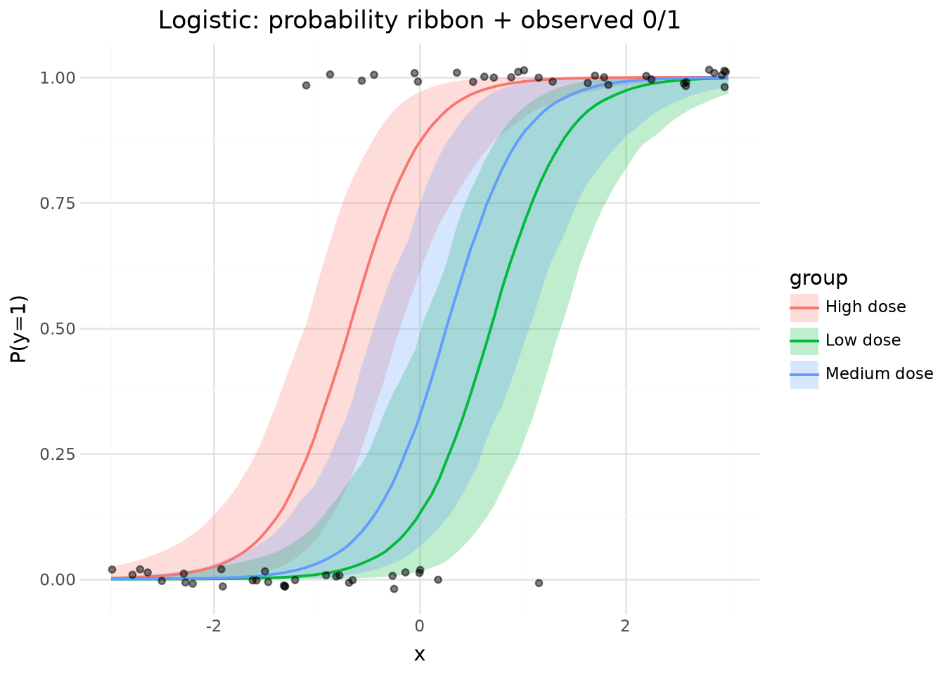
# 6. Logistic regression
Bernoulli outcome with group-level intercepts. Predictions are computed directly from parameter draws by joining `alpha[group]` and `beta` with the prediction grid -- no `sample_posterior_predictive` needed. Exercises [parameter_draws](../../reference/parameter_draws.md#tidydraws.parameter_draws) with a non-gaussian model and demonstrates manual prediction computation.
``` python
dt, obs, grid = logistic(seed=2031)
```
Initializing NUTS using jitter+adapt_diag...
Multiprocess sampling (2 chains in 2 jobs)
NUTS: [alpha, beta]
Sampling 2 chains for 400 tune and 400 draw iterations (800 + 800 draws total) took 1 seconds.
We recommend running at least 4 chains for robust computation of convergence diagnostics
## Use tidydraws
``` python
draws = td.parameter_draws(dt, "alpha", "beta")
```
Cross-join detected between frame 0 and 1. Broadcasting scalar or differently-dimensioned variable on dims ['chain', 'draw'].
``` python
# Compute predictions: join draws with grid, then logit_p → p
pred_draws = draws.join(grid.select(["obs_ind", "group", "x"]), on="group")
pred_draws = pred_draws.with_columns(
(1 / (1 + (-pl.col("alpha") - pl.col("beta") * pl.col("x")).exp())).alias("p"),
)
pred_summary = td.point_interval(
pred_draws, "p", group_by=["obs_ind", "x", "group"], probs=(0.80, 0.95)
)
```
- lets-plot
- plotnine
``` python
(
lp.ggplot(
pred_summary.to_pandas(),
lp.aes("x"),
)
+ lp.geom_ribbon(
lp.aes(ymin="p_lower_0.95", ymax="p_upper_0.95", fill="group"), alpha=0.25
)
+ lp.geom_line(lp.aes(y="p", color="group"), size=0.8)
+ lp.geom_jitter(
lp.aes(y="y"),
data=obs.with_columns(pl.col("y").cast(pl.Float64)).to_pandas(),
alpha=0.5,
height=0.02,
size=1.5,
)
+ lp.labs(
x="x",
y="P(y=1)",
color="group",
fill="group",
title="Logistic: probability ribbon + observed 0/1",
)
+ lp.theme_minimal()
)
```
``` python
(
p9.ggplot(
pred_summary.to_pandas(),
p9.aes("x"),
)
+ p9.geom_ribbon(
p9.aes(ymin="p_lower_0.95", ymax="p_upper_0.95", fill="group"), alpha=0.25
)
+ p9.geom_line(p9.aes(y="p", color="group"), size=0.8)
+ p9.geom_jitter(
p9.aes(y="y"),
data=obs.with_columns(pl.col("y").cast(pl.Float64)).to_pandas(),
alpha=0.5,
height=0.02,
size=1.5,
)
+ p9.labs(
x="x",
y="P(y=1)",
color="group",
fill="group",
title="Logistic: probability ribbon + observed 0/1",
)
+ p9.theme_minimal()
)
```
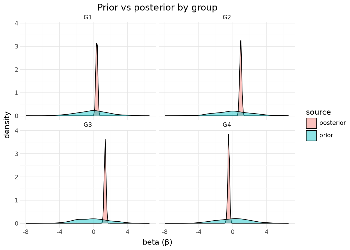
# 7. Prior vs posterior
[compare_draws()](../../reference/compare_draws.md#tidydraws.compare_draws) stacks prior and posterior into one frame with a `source` column. Exercises the stacked-concat path with real PyMC prior samples.
``` python
dt, _obs = varying_slopes(seed=2028) # same seed as §3 -- already has prior
```
Sampling: [alpha, beta, sigma]
Initializing NUTS using jitter+adapt_diag...
Multiprocess sampling (2 chains in 2 jobs)
NUTS: [alpha, beta, sigma]
Sampling 2 chains for 400 tune and 400 draw iterations (800 + 800 draws total) took 0 seconds.
We recommend running at least 4 chains for robust computation of convergence diagnostics
The rhat statistic is larger than 1.01 for some parameters. This indicates problems during sampling. See https://arxiv.org/abs/1903.08008 for details
## Use tidydraws
``` python
compare = td.compare_draws(dt, "beta", groups=["prior", "posterior"])
```
## Overlaid prior and posterior densities
- lets-plot
- plotnine
``` python
(
lp.ggplot(compare.to_pandas(), lp.aes("beta", fill="source"))
+ lp.geom_density(alpha=0.45)
+ lp.facet_wrap(facets="group", ncol=2)
+ lp.labs(
x="beta (β)", y="density", fill="source", title="Prior vs posterior by group"
)
+ lp.theme_minimal()
)
```
``` python
(
p9.ggplot(compare.to_pandas(), p9.aes("beta", fill="source"))
+ p9.geom_density(alpha=0.45)
+ p9.facet_wrap("~group", ncol=2)
+ p9.labs(
x="beta (β)", y="density", fill="source", title="Prior vs posterior by group"
)
+ p9.theme_minimal()
)
```
# 8. Single chain
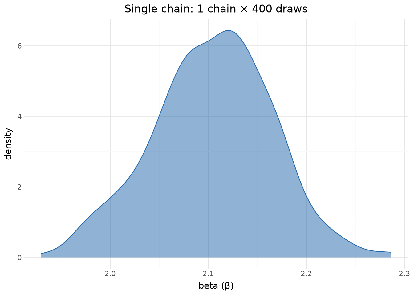
Same simple regression as §1, but sampled with `chains=1`. Verifies that nothing in the extraction or alignment assumes `chain >= 2`.
``` python
dt, obs = simple_regression_1chain(seed=2032)
```
Initializing NUTS using jitter+adapt_diag...
Sequential sampling (1 chains in 1 job)
NUTS: [alpha, beta, sigma]
Sampling 1 chain for 400 tune and 400 draw iterations (400 + 400 draws total) took 0 seconds.
Only one chain was sampled, this makes it impossible to run some convergence checks
## Use tidydraws
``` python
draws = td.parameter_draws(dt, "alpha", "beta", "sigma")
```
Cross-join detected between frame 0 and 1. Broadcasting scalar or differently-dimensioned variable on dims ['chain', 'draw'].
Cross-join detected between frame 1 and 2. Broadcasting scalar or differently-dimensioned variable on dims ['chain', 'draw'].
## Density with one chain
- lets-plot
- plotnine
``` python
(
lp.ggplot(draws.to_pandas(), lp.aes("beta"))
+ lp.geom_density(fill="#2166ac", alpha=0.5, color="#2166ac")
+ lp.labs(
x="beta (β)",
y="density",
title=f"Single chain: {draws.select(pl.col('chain').n_unique()).item()} chain × {draws.select(pl.col('draw').n_unique()).item()} draws",
)
+ lp.theme_minimal()
)
```
``` python
(
p9.ggplot(draws.to_pandas(), p9.aes("beta"))
+ p9.geom_density(fill="#2166ac", alpha=0.5, color="#2166ac")
+ p9.labs(
x="beta (β)",
y="density",
title=f"Single chain: {draws.select(pl.col('chain').n_unique()).item()} chain × {draws.select(pl.col('draw').n_unique()).item()} draws",
)
+ p9.theme_minimal()
)
```