Imagine you ran a clean lift test on one of your channels. The experimental estimate is precise, the MMM calibration works, and the obvious stakeholder question arrives:
Great. So now we know the incremental ROAS and the saturation ceiling for this channel, right?
That sounds plausible, but it is usually too strong a claim. A lift test gives you local causal evidence about the response near the spend level you tested. But recovering both things the practitioner wants — the steepness \(\lambda\), which drives incremental ROAS, and the ceiling \(\beta\), which sets the channel’s absolute contribution — requires more than one local measurement. The ceiling only reveals itself far out in the tail of the curve, well beyond the operating point of a typical lift test.
This post is about that distinction. I will use the two-parameter logistic saturation formulation used in PyMC-Marketing and show why a single lift test is best understood as a local anchor rather than a joint estimator of both parameters. If we want to learn about the ceiling, we need a ladder of experiments at different spend levels that probe different parts of the curve.
A lift test is a local measurement
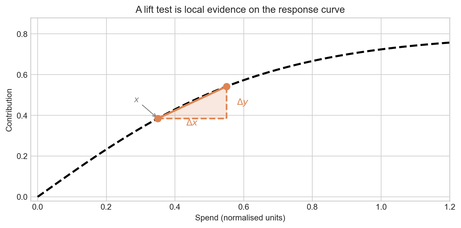
A lift test does not observe the whole curve. It observes a difference between two operating points:
\[ \Delta y = f(x + \Delta x) - f(x) \]
That is easiest to see geometrically: a lift test is a little triangle sitting on the saturation curve. The base is \(\Delta x\), the height is \(\Delta y\), and the operating point is the baseline spend \(x\).
In other words, a lift test directly measures the incremental return on ad-spend (iROAS) at the tested operating point — the ratio of the revenue increment to the spend increment:
\[ \text{iROAS} = \frac{\Delta y}{\Delta x} = \frac{f(x + \Delta x) - f(x)}{\Delta x} \]
This is an average slope between two spend levels. Its value depends on where on the curve you are (\(x\)) and how large a step you took (\(\Delta x\)). If you care about incremental ROAS near the spend level you tested, a lift test is excellent.
But the asymptote is different: it is a statement about where the curve eventually plateaus, far out in the tail — a region the lift test never touched.
One clean lift test is consistent with many different ceilings
In this parameterization, the same lift can be written as
\[ \Delta y = \beta \cdot \left[h(\lambda, x + \Delta x) - h(\lambda, x)\right] \]
where
\[ h(\lambda, x) = \frac{1 - e^{-\lambda x}}{1 + e^{-\lambda x}}. \]
Now hold \(x\), \(\Delta x\), and \(\Delta y\) fixed. You still have one equation involving two unknowns: \(\lambda\) and \(\beta\). That is the heart of the problem.
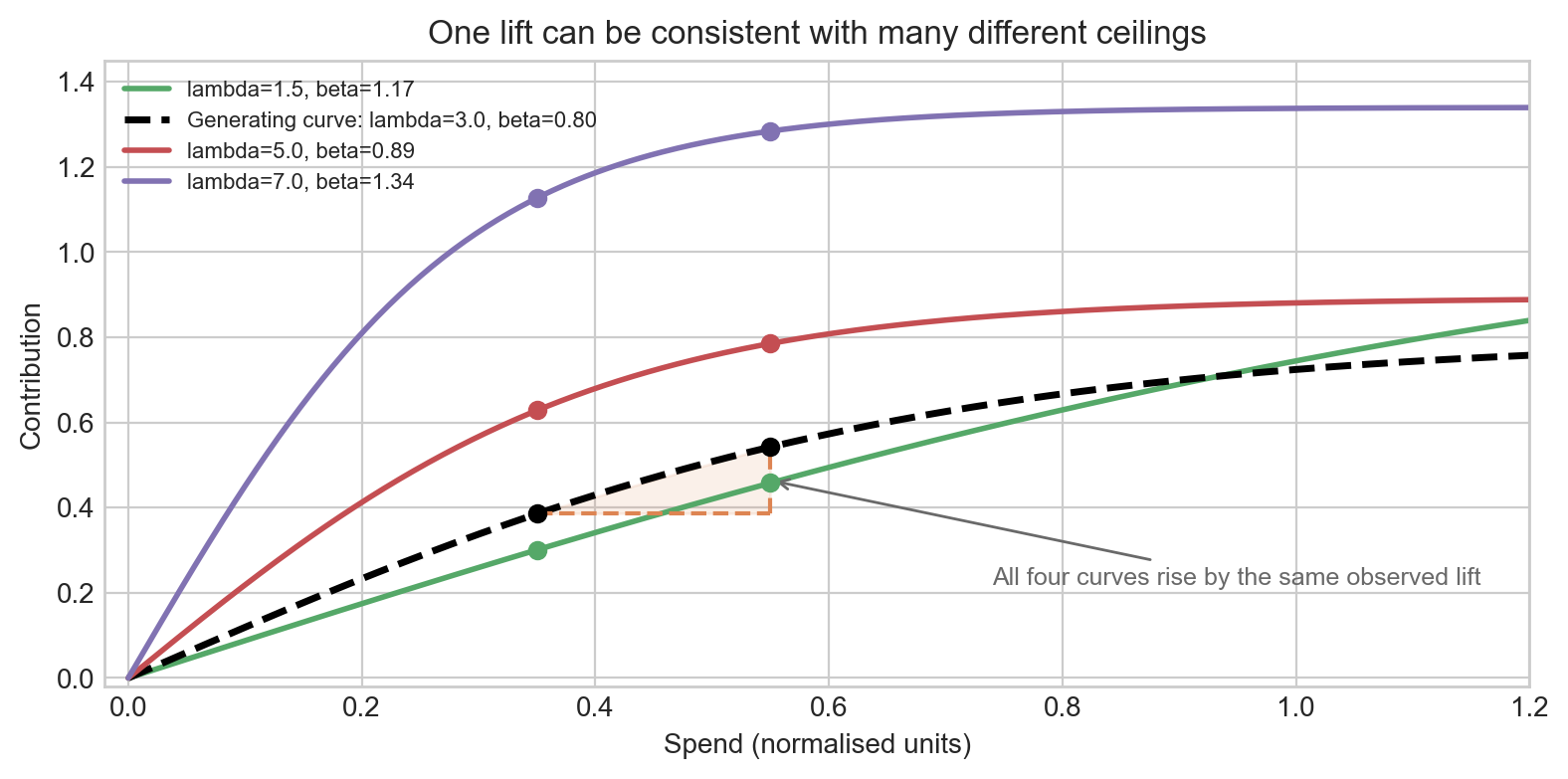
Figure 2 is the key intuition. A shallow curve with a larger ceiling can fit the same local rise as a steeper curve with a smaller ceiling. A single lift test rules out a lot of nonsense, but it does not usually collapse the problem to one unique ceiling.
The same story in parameter space
The cleanest way to see this is to move from curve space to parameter space. For a fixed lift test, every compatible pair satisfies
\[ \beta(\lambda) = \frac{\Delta y}{h(\lambda, x + \Delta x) - h(\lambda, x)}. \]
Here \(\beta(\lambda)\) is read as the ceiling value implied by a particular choice of \(\lambda\), given the fixed observed lift \(\Delta y\). For every value of \(\lambda\) you might consider, this formula tells you the unique \(\beta\) that would reproduce that same lift — so together they trace out a curve rather than a single point.
That is not a single point. It is a whole curve in \((\lambda, \beta)\) space.
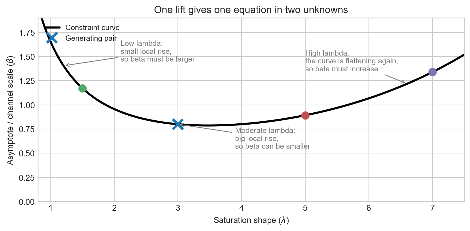
NoteA useful mental model
One lift test gives you a constraint curve in \((\lambda, \beta)\) space — not a point estimate for either parameter. With realistic measurement noise, that knife-edge curve broadens into a probability ridge, as we formalise below. That is why a single clean experiment can still leave substantial uncertainty about both the shape and the ceiling, even when it is highly informative about the local response near the tested spend level.
The picture in Figure 3 is also a nice antidote to a common misconception. If the posterior asymptote happens to look reasonable after one lift test, that does not mean the lift by itself identified the ceiling. More often, the lift has carved out a sensible ridge and the rest of the model – observational likelihood, priors, and functional form – has done the rest.
A second lift changes the game
Now add a second experiment at a meaningfully different operating point. That gives you a second equation and therefore a second constraint curve.
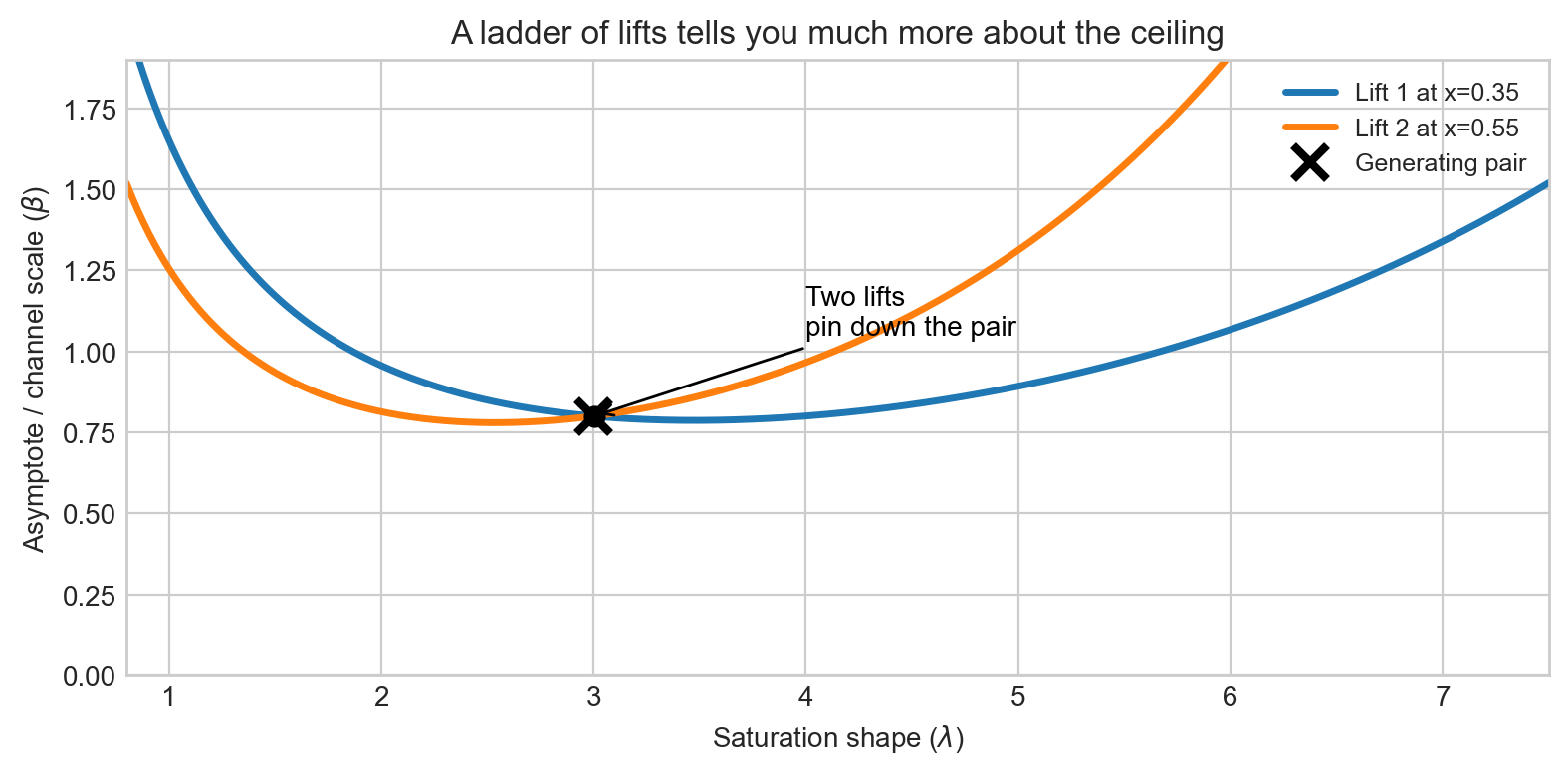
This is the real design insight. If your scientific question is about the asymptote, then the relevant experimental program is not “run one lift.” It is closer to “run a ladder of lifts that probes different parts of the curve.”
In practice, the most informative pair is often something like:
- one lift in a steeper region of the curve,
- and another at a meaningfully higher spend where diminishing returns are more pronounced.
That does not magically solve every identification problem, but it moves you much closer to learning the global shape rather than just the local slope.
From exact geometry to realistic uncertainty
The constraint curves above assume the lift is observed exactly — a clean, noise-free number. In practice, a lift test is an experiment with uncertainty. The exact causal change in our outcome attributable to the lift is not known with certainty, which means \(\hat{\Delta y}\) carries uncertainty.
Model the observed lift as \(\hat{\Delta y} \sim \mathcal{N}\!\left(\Delta y(\lambda, \beta),\; \sigma^2\right)\), where the true increment \(\Delta y(\lambda, \beta) = \beta \cdot [h(\lambda, x + \Delta x) - h(\lambda, x)]\) depends on the parameters. For every point on a fine grid over \((\lambda, \beta)\) we can evaluate the log-likelihood
\[ \log p(\hat{\Delta y} \mid \lambda, \beta) = -\frac{1}{2}\left(\frac{\hat{\Delta y} - \Delta y(\lambda, \beta)}{\sigma}\right)^2 + \text{const} \]
and display the result as a heatmap. The constraint curve from the previous section corresponds to the limiting case \(\sigma \to 0\); for a realistic experiment it becomes a probability ridge — a band of high relative likelihood aligned along the direction of degeneracy.
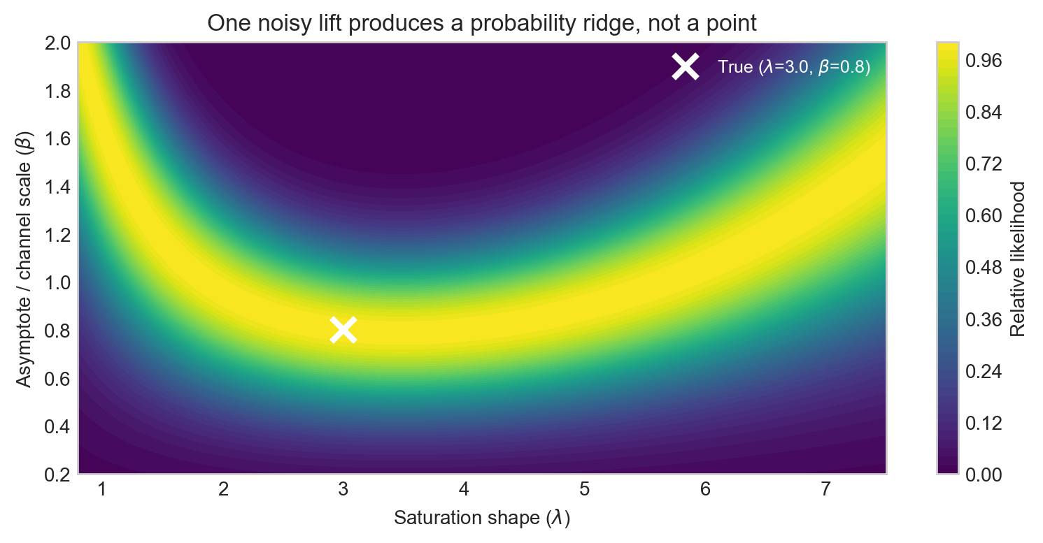
The ridge in Figure 5 is wide along the \((\lambda, \beta)\) degeneracy direction and narrow perpendicular to it. The single test is very informative about one specific combination of the two parameters — essentially the incremental ROAS at the tested spend level — but barely constrains the orthogonal combination, which is closer to the global ceiling.
Adding a second lift at a different operating point gives a second likelihood surface. Summing the log-likelihoods gives the joint surface for both experiments together.
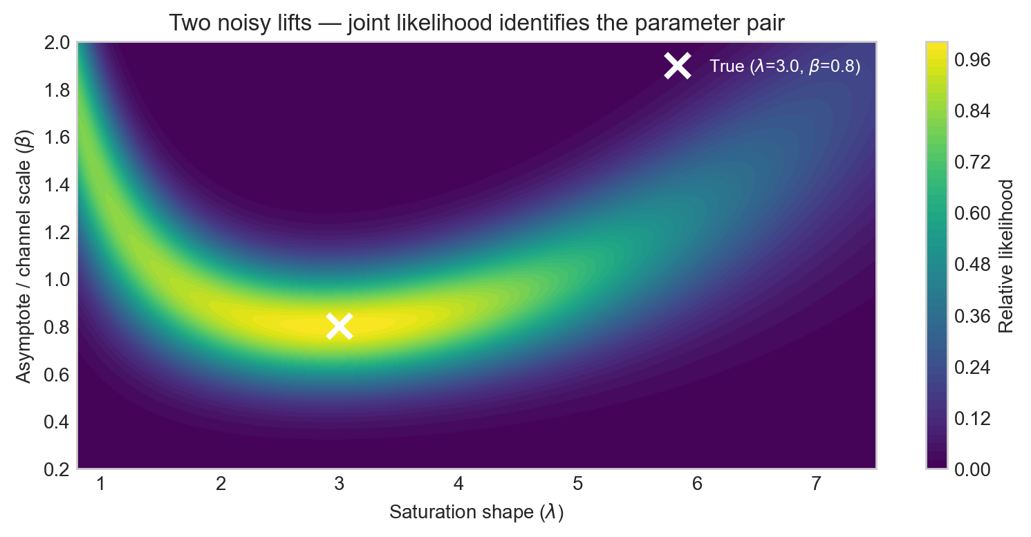
Figure 6 shows the key result in probabilistic terms: two lifts from well-separated operating points triangulate the true pair far more tightly than either experiment alone. This is the realistic, noisy version of the exact constraint-curve intersection in Figure 4.
NoteThe ridge direction tells you what is and is not learnable
Each likelihood ridge runs roughly along the direction in \((\lambda, \beta)\) space that preserves the incremental ROAS at the tested spend level. That direction is what the experiment cannot distinguish on its own. A second experiment at a different spend level has a ridge running in a different direction, and their intersection is where the real information lies.
What the MMM adds, and what it does not
A calibrated MMM does add real information
The toy geometry above intentionally isolates the experiment. A real MMM does not work that way — it combines the experimental constraint with two other sources of information: a prior over \((\lambda, \beta)\) and an observational likelihood from the historical spend-and-revenue time series. Each source carves out its own region of plausible parameter values, and the joint posterior is the overlap of all three.
This means a well-specified MMM can produce a meaningfully tighter posterior for \(\beta\) than the lift test alone would suggest. That is not a flaw — it is the point of building a model. The key word is joint: the tightening comes from combining sources, not from the lift test having resolved the ambiguity on its own.
But precision is not the same as experimental identification
Imagine you feed one lift test into a full MMM and the posterior for \(\beta\) comes back looking tight and plausible — maybe even centred close to the true ceiling. It is tempting to conclude that the lift test identified the ceiling. But this can be misleading, because the posterior’s apparent precision may have come from sources that have nothing to do with the experiment:
- The prior. If the prior on \(\beta\) is narrow, the posterior will be narrow regardless of what the data say. The lift has not done the work; the prior has.
- Observational model structure. The MMM also fits historical spend-and-revenue time series. Tight correlations in that observational data can sharpen the posterior, but observational co-variation is not the same as causal identification. Spend and revenue move together for many reasons besides the true saturation relationship.
The likelihood heatmaps in this post are a useful benchmark precisely because they isolate what the experiment alone tells you. A lifted spend was randomly assigned, so the resulting \(\Delta y\) is causally clean. The width and orientation of that likelihood ridge is an honest picture of experimental information about \((\lambda, \beta)\). If the full MMM posterior looks substantially tighter than that ridge, you should ask why — and the answer is almost always prior choice or observational model structure, not the lift test itself.
A confident-looking posterior that happens to be near the truth is not the same as having genuinely learned the answer from data. Getting the right answer for the wrong reason is a fragile state: it will not generalise reliably when the prior is misspecified or when the observational correlations shift.
This is why the parameter-space and likelihood plots in this post are worth examining carefully. They make the residual ambiguity from the experiment visible, and show exactly where the rest of the model — priors and observational structure — is still doing the heavy lifting.
Takeaways for practitioners
- Single lift: great for estimating incremental ROAS at the tested operating point; one equation in two unknowns (\(\lambda\), \(\beta\)).
- Likelihood ridge: with realistic measurement noise, the constraint curve broadens into a probability band in \((\lambda, \beta)\) space.
- Asymptote \(\beta\): a global property of the curve, not recoverable from a single local measurement alone.
- Saturation shape \(\lambda\): controls the steepness of the saturation curve, and therefore incremental ROAS; not individually pinned by a single lift.
- Ladder of lifts: if you care about either the ceiling or the saturation shape, design experiments spanning different spend levels — joint likelihoods triangulate the pair.
- Joint identification: when a calibrated MMM tightens the asymptote after one lift, the observational model and priors are contributing too.
If you had budget for exactly one more experiment, where would you place it: near your current spend, or deliberately at a very different operating point to learn more about the curve’s tail?