Prior/posterior comparison

Fit a PyMC model, compare prior and posterior draws with compare_draws(), and plot them

compare_draws() is the prior/posterior comparison helper: it calls parameter_draws() once per selected group in the ArviZ object, tags each result with a source column, and stacks them into a single DataFrame. By default it compares posterior against prior, which is the workflow most users need after fitting a PyMC model.

Full PyMC workflow

This example uses the same grouped regression data as the other examples, samples from the model prior before fitting, then compares those prior draws with the fitted posterior. That gives compare_draws() real prior draws and real posterior draws from the same PyMC model.

Code

from pathlib import Path
import sys

import polars as pl
import pymc as pm
import tidydraws as td
import lets_plot as lp
import plotnine as p9


for parent in [Path.cwd(), *Path.cwd().parents]:
    helper_dir = parent / "docs" / "examples"
    if (helper_dir / "_pymc_workflow.py").exists():
        sys.path.insert(0, str(helper_dir))
        break

from _pymc_workflow import simulate_grouped_regression

lp.LetsPlot.setup_html()

workflow = simulate_grouped_regression(seed=2026)
observed = workflow.observed
truth = workflow.truth

/home/runner/work/tidydraws/tidydraws/.venv/lib/python3.12/site-packages/lets_plot/plot/annotation.py:551: SyntaxWarning: invalid escape sequence '\('
  """
/home/runner/work/tidydraws/tidydraws/.venv/lib/python3.12/site-packages/lets_plot/plot/annotation.py:601: SyntaxWarning: invalid escape sequence '\('
  """

Build our PyMC model and fit.

coords = {
    "groups": workflow.group_names,
    "obs_ind": observed.get_column("obs_ind").to_numpy(),
}

with pm.Model(coords=coords) as model:
    x = pm.Data("x", observed.get_column("x").to_numpy(), dims="obs_ind")
    group_idx = pm.Data(
        "group_idx",
        observed.get_column("group_idx").to_numpy().astype("int64"),
        dims="obs_ind",
    )
    intercept = pm.Normal("intercept", mu=0.0, sigma=2.0, dims="groups")
    beta = pm.Normal("beta", mu=0.0, sigma=1.5, dims="groups")
    sigma = pm.HalfNormal("sigma", sigma=1.0)
    mu = pm.Deterministic(
        "mu",
        intercept[group_idx] + beta[group_idx] * x,
        dims="obs_ind",
    )
    pm.Normal(
        "y",
        mu=mu,
        sigma=sigma,
        observed=observed.get_column("y").to_numpy(),
        dims="obs_ind",
    )
    prior = pm.sample_prior_predictive(
        draws=800,
        random_seed=2029,
        var_names=["intercept", "beta", "sigma"],
    )
    dt = pm.sample(
        draws=400,
        random_seed=2030,
    )

    # arviz 1.0+ uses .update(), 0.x uses .extend()
    try:
        dt.update(prior)
    except AttributeError:
        dt.extend(prior)

Sampling: [beta, intercept, sigma]
Initializing NUTS using jitter+adapt_diag...
Multiprocess sampling (2 chains in 2 jobs)
NUTS: [intercept, beta, sigma]

Sampling 2 chains for 1_000 tune and 400 draw iterations (2_000 + 800 draws total) took 1 seconds.
We recommend running at least 4 chains for robust computation of convergence diagnostics

dt

Use tidydraws

One call stacks both sources:

compare = td.compare_draws(dt, "beta")
compare.head()

shape: (5, 5)

chain	draw	groups	beta	source
i64	i64	str	f64	str
0	0	"North"	0.394303	"posterior"
0	0	"South"	0.782	"posterior"
0	0	"East"	1.384254	"posterior"
0	0	"West"	-0.407587	"posterior"
0	1	"North"	0.473318	"posterior"

Plotting

Prior vs posterior (pooled)

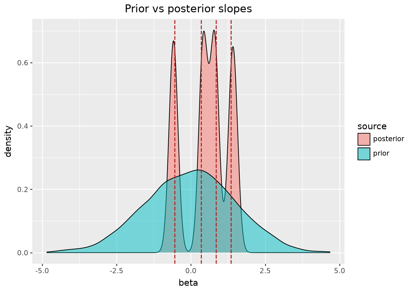
The prior is deliberately broad; after seeing the data, the posterior concentrates around the group-specific slopes.

(
    lp.ggplot(compare.to_pandas(), lp.aes("beta", fill="source"))
    + lp.geom_density(alpha=0.5)
    + lp.geom_vline(
        data=truth.to_pandas(),
        mapping=lp.aes(xintercept="beta_true"),
        color="firebrick",
        linetype="dashed",
        size=0.7,
    )
    + lp.labs(x="beta", y="density", fill="source", title="Prior vs posterior slopes")
)

Prior vs posterior density of group-specific slopes, pooled across groups.

(
    p9.ggplot(compare.to_pandas(), p9.aes("beta", fill="source"))
    + p9.geom_density(alpha=0.5)
    + p9.geom_vline(
        data=truth.to_pandas(),
        mapping=p9.aes(xintercept="beta_true"),
        color="firebrick",
        linetype="dashed",
        size=0.7,
    )
    + p9.labs(x="beta", y="density", fill="source", title="Prior vs posterior slopes")
)

Prior vs posterior by group

(
    lp.ggplot(compare.to_pandas(), lp.aes("beta", fill="source"))
    + lp.geom_density(alpha=0.5)
    + lp.geom_vline(
        data=truth.to_pandas(),
        mapping=lp.aes(xintercept="beta_true"),
        color="firebrick",
        linetype="dashed",
        size=0.7,
    )
    + lp.facet_wrap(facets="groups", ncol=2)
    + lp.labs(x="beta", y="density", fill="source", title="Prior vs posterior by group")
)

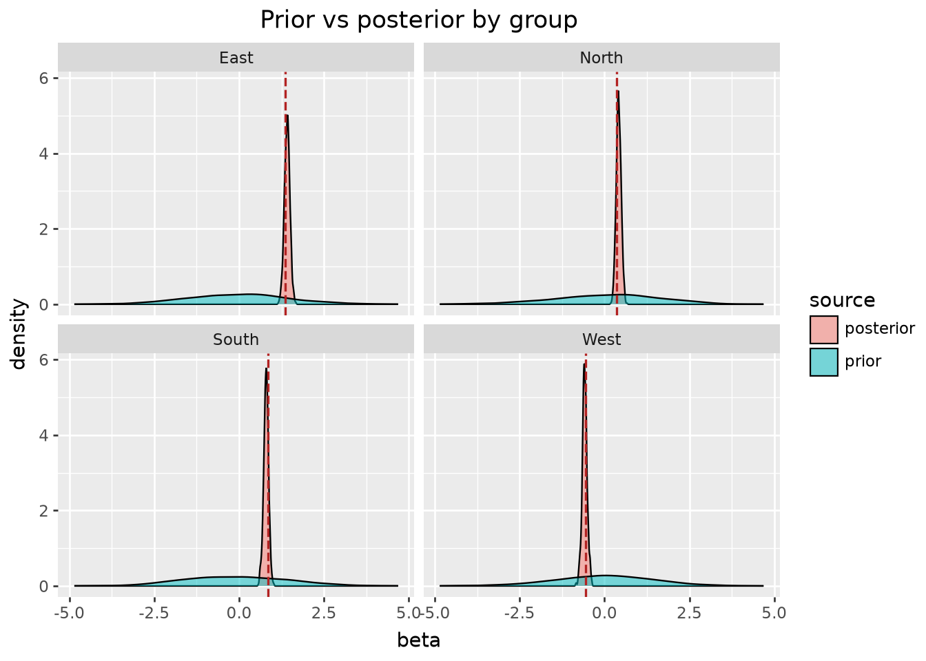
Prior vs posterior density of group-specific slopes, faceted by group.

(
    p9.ggplot(compare.to_pandas(), p9.aes("beta", fill="source"))
    + p9.geom_density(alpha=0.5)
    + p9.geom_vline(
        data=truth.to_pandas(),
        mapping=p9.aes(xintercept="beta_true"),
        color="firebrick",
        linetype="dashed",
        size=0.7,
    )
    + p9.facet_wrap("~groups", ncol=2)
    + p9.labs(x="beta", y="density", fill="source", title="Prior vs posterior by group")
)

Credible-interval comparison

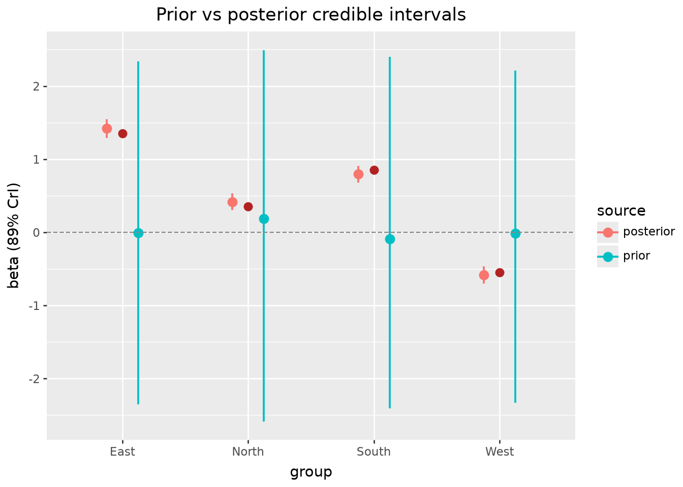
A different cut: 89% intervals per group, dodged by source. The posterior intervals contract toward the true slopes while the prior intervals remain wide.

ci = td.point_interval(compare, "beta", group_by=["groups", "source"], probs=(0.89,))

(
    lp.ggplot(ci.to_pandas(), lp.aes("groups", "beta", color="source"))
    + lp.geom_pointrange(
        lp.aes(ymin="beta_lower", ymax="beta_upper"),
        position=lp.position_dodge(0.5),
        size=0.8,
    )
    + lp.geom_pointrange(
        data=truth.to_pandas(),
        mapping=lp.aes("groups", "beta_true", ymin="beta_true", ymax="beta_true"),
        color="firebrick",
        size=0.7,
    )
    + lp.geom_hline(yintercept=0, linetype="dashed", color="#888888")
    + lp.labs(
        x="group",
        y="beta (89% CrI)",
        color="source",
        title="Prior vs posterior credible intervals",
    )
)

Prior vs posterior 89% credible intervals of group-specific slopes.

(
    p9.ggplot(ci.to_pandas(), p9.aes("groups", "beta", color="source"))
    + p9.geom_pointrange(
        p9.aes(ymin="beta_lower", ymax="beta_upper"),
        position=p9.position_dodge(0.5),
        size=0.8,
    )
    + p9.geom_pointrange(
        data=truth.to_pandas(),
        mapping=p9.aes("groups", "beta_true", ymin="beta_true", ymax="beta_true"),
        color="firebrick",
        size=0.7,
    )
    + p9.geom_hline(yintercept=0, linetype="dashed", color="#888888")
    + p9.labs(
        x="group",
        y="beta (89% CrI)",
        color="source",
        title="Prior vs posterior credible intervals",
    )
)

group_name sets the source column’s name, and groups can compare other ArviZ groups when needed. Next, join posterior expectations to covariates with prediction_draws().