Parameter space

Fit a PyMC model, extract posterior draws with parameter_draws(), and plot them

parameter_draws() is the entry point for parameter-space plots: it pulls posterior draws out of an ArviZ object into a tidy Polars DataFrame — one row per chain × draw × coordinate, each variable a column. This example starts with simulated observed data, fits a real PyMC model, and then uses the resulting posterior draws for densities, intervals, contrasts, and cross-parameter plots.

Full PyMC workflow

The data are generated from four groups with deliberately different intercepts and slopes, including one negative slope. That separation makes the posterior plots diagnose real group differences rather than noise around one common line.

Code

from pathlib import Path
import sys

import numpy as np
import polars as pl
import pymc as pm
import tidydraws as td
import lets_plot as lp
import plotnine as p9

for parent in [Path.cwd(), *Path.cwd().parents]:
    helper_dir = parent / "docs" / "examples"
    if (helper_dir / "_pymc_workflow.py").exists():
        sys.path.insert(0, str(helper_dir))
        break

from _pymc_workflow import simulate_grouped_regression

lp.LetsPlot.setup_html()

workflow = simulate_grouped_regression(seed=2026)
observed = workflow.observed
truth = workflow.truth

The observed data and true generating lines show the group separation before fitting.

(
    lp.ggplot(observed.sort(["groups", "x"]).to_pandas(), lp.aes("x", "y"))
    + lp.geom_point(lp.aes(color="groups"), alpha=0.65, size=2.0)
    + lp.geom_line(lp.aes(y="mu_true", color="groups"), size=1.0)
    + lp.labs(
        x="x", y="y", color="group", title="Observed data from known group differences"
    )
)

Simulated observed data with true group-specific regression lines.

Now we build our PyMC model and fit.

coords = {
    "groups": workflow.group_names,
    "obs_ind": observed.get_column("obs_ind").to_numpy(),
}

with pm.Model(coords=coords) as model:
    x = pm.Data("x", observed.get_column("x").to_numpy(), dims="obs_ind")
    group_idx = pm.Data(
        "group_idx",
        observed.get_column("group_idx").to_numpy().astype("int64"),
        dims="obs_ind",
    )
    intercept = pm.Normal("intercept", mu=0.0, sigma=2.0, dims="groups")
    beta = pm.Normal("beta", mu=0.0, sigma=1.5, dims="groups")
    sigma = pm.HalfNormal("sigma", sigma=1.0)
    mu = pm.Deterministic(
        "mu",
        intercept[group_idx] + beta[group_idx] * x,
        dims="obs_ind",
    )
    pm.Normal(
        "y",
        mu=mu,
        sigma=sigma,
        observed=observed.get_column("y").to_numpy(),
        dims="obs_ind",
    )
    dt = pm.sample(
        draws=400,
        tune=400,
        random_seed=2026,
    )

Initializing NUTS using jitter+adapt_diag...
Multiprocess sampling (2 chains in 2 jobs)
NUTS: [intercept, beta, sigma]

Sampling 2 chains for 400 tune and 400 draw iterations (800 + 800 draws total) took 1 seconds.
We recommend running at least 4 chains for robust computation of convergence diagnostics
The rhat statistic is larger than 1.01 for some parameters. This indicates problems during sampling. See https://arxiv.org/abs/1903.08008 for details

dt

Use tidydraws

One parameter_draws() call extracts group slopes and intercepts from the fitted posterior:

beta_df = td.parameter_draws(dt, "beta", "intercept")
beta_df.head()

shape: (5, 5)

chain	draw	groups	beta	intercept
i64	i64	str	f64	f64
0	0	"North"	0.356443	-1.365803
0	0	"South"	0.647371	0.253135
0	0	"East"	1.384258	1.345093
0	0	"West"	-0.538669	2.264232
0	1	"North"	0.505888	-1.138709

Plotting

Posterior density by group

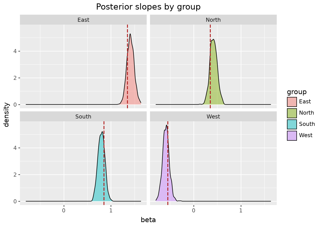
The dashed red lines are the true slopes used to simulate the data.

(
    lp.ggplot(beta_df.to_pandas(), lp.aes("beta", fill="groups"))
    + lp.geom_density(alpha=0.45)
    + lp.geom_vline(
        data=truth.to_pandas(),
        mapping=lp.aes(xintercept="beta_true"),
        color="firebrick",
        linetype="dashed",
        size=0.8,
    )
    + lp.facet_wrap(facets="groups", ncol=2)
    + lp.labs(x="beta", y="density", fill="group", title="Posterior slopes by group")
)

Posterior density of group-specific slopes, with true values marked.

(
    p9.ggplot(beta_df.to_pandas(), p9.aes("beta", fill="groups"))
    + p9.geom_density(alpha=0.45)
    + p9.geom_vline(
        data=truth.to_pandas(),
        mapping=p9.aes(xintercept="beta_true"),
        color="firebrick",
        linetype="dashed",
        size=0.8,
    )
    + p9.facet_wrap("~groups", ncol=2)
    + p9.labs(x="beta", y="density", fill="group", title="Posterior slopes by group")
)

Forest plot

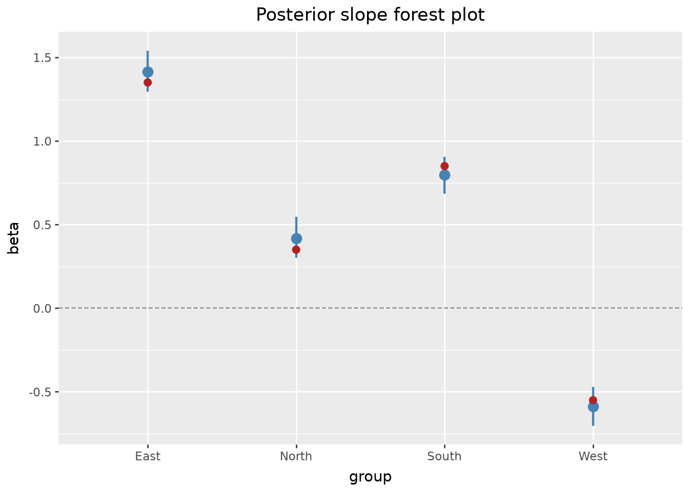
Summarise each group with one central 89% interval. The red points are the true slopes used to generate the observed data.

beta_forest = td.point_interval(beta_df, "beta", group_by="groups", probs=(0.89,))

(
    lp.ggplot(beta_forest.to_pandas(), lp.aes("groups", "beta"))
    + lp.geom_pointrange(
        lp.aes(ymin="beta_lower", ymax="beta_upper"),
        color="steelblue",
        size=0.9,
    )
    + lp.geom_point(
        data=truth.to_pandas(),
        mapping=lp.aes("groups", "beta_true"),
        color="firebrick",
        size=2.4,
    )
    + lp.geom_hline(yintercept=0, linetype="dashed", color="#888888")
    + lp.labs(x="group", y="beta", title="Posterior slope forest plot")
)

Posterior slope forest plot with 89% intervals and true values.

(
    p9.ggplot(beta_forest.to_pandas(), p9.aes("groups", "beta"))
    + p9.geom_pointrange(
        p9.aes(ymin="beta_lower", ymax="beta_upper"),
        color="steelblue",
        size=0.9,
    )
    + p9.geom_point(
        data=truth.to_pandas(),
        mapping=p9.aes("groups", "beta_true"),
        color="firebrick",
        size=2.4,
    )
    + p9.geom_hline(yintercept=0, linetype="dashed", color="#888888")
    + p9.labs(x="group", y="beta", title="Posterior slope forest plot")
)

Quantile dotplot

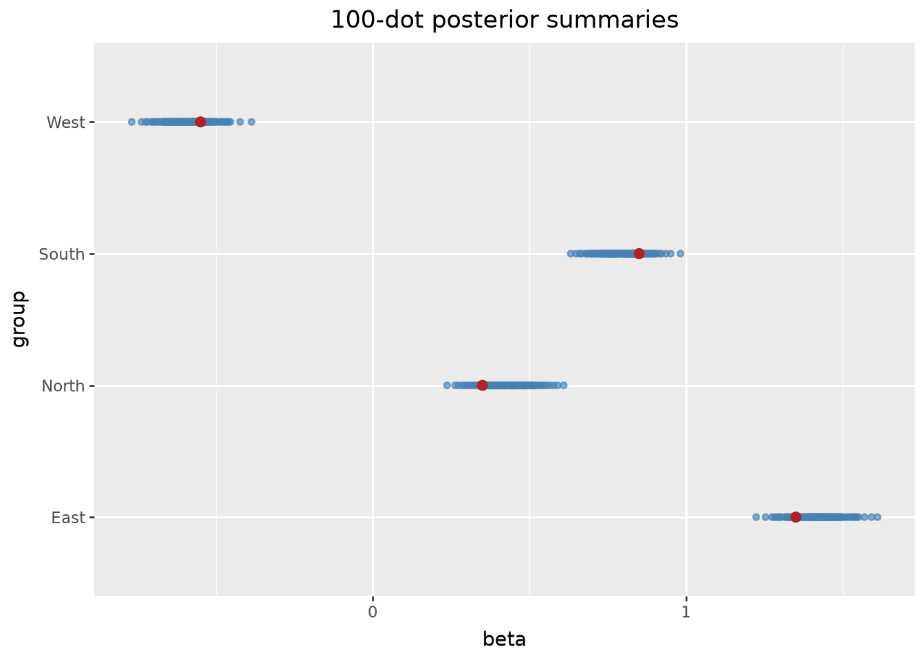
Each row below has 100 equally likely dots from the posterior slope distribution for a group. This is a frequency-format alternative to density plots.

quantiles = np.linspace(0.005, 0.995, 100)
group_levels = (
    beta_df.select("groups").unique().sort("groups").get_column("groups").to_list()
)
quantile_dots = pl.DataFrame([
    {
        "groups": group_name,
        "beta": float(
            beta_df
            .filter(pl.col("groups") == group_name)
            .get_column("beta")
            .quantile(q)
        ),
        "dot": dot,
    }
    for group_name in group_levels
    for dot, q in enumerate(quantiles, start=1)
])

(
    lp.ggplot(quantile_dots.to_pandas(), lp.aes("beta", "groups"))
    + lp.geom_point(size=1.4, alpha=0.65, color="steelblue")
    + lp.geom_point(
        data=truth.to_pandas(),
        mapping=lp.aes("beta_true", "groups"),
        color="firebrick",
        size=2.4,
    )
    + lp.labs(x="beta", y="group", title="100-dot posterior summaries")
)

Quantile dotplot of group-specific slopes: each dot represents 1% posterior mass.

(
    p9.ggplot(quantile_dots.to_pandas(), p9.aes("beta", "groups"))
    + p9.geom_point(size=1.4, alpha=0.65, color="steelblue")
    + p9.geom_point(
        data=truth.to_pandas(),
        mapping=p9.aes("beta_true", "groups"),
        color="firebrick",
        size=2.4,
    )
    + p9.labs(x="beta", y="group", title="100-dot posterior summaries")
)

Derived contrasts against a reference group

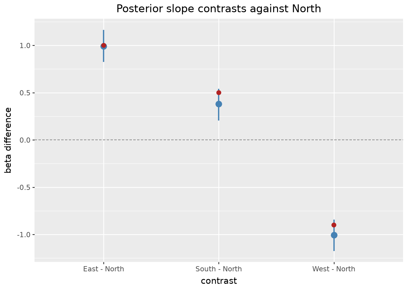
Because every row keeps its chain and draw, derived quantities are ordinary dataframe operations. Here each contrast is beta[group] - beta[North] within draw, summarised with one 89% interval.

reference_group = "North"
wide_beta = beta_df.pivot(index=["chain", "draw"], on="groups", values="beta")
contrast_draws = pl.concat([
    wide_beta.select(
        "chain",
        "draw",
        (pl.col(group_name) - pl.col(reference_group)).alias("contrast"),
        pl.lit(f"{group_name} - {reference_group}").alias("contrast_name"),
    )
    for group_name in group_levels
    if group_name != reference_group
])
contrast_forest = td.point_interval(
    contrast_draws, "contrast", group_by="contrast_name", probs=(0.89,)
)
reference_truth = truth.filter(pl.col("groups") == reference_group).get_column(
    "beta_true"
)[0]
truth_contrasts = truth.filter(pl.col("groups") != reference_group).select(
    (pl.col("groups") + " - " + pl.lit(reference_group)).alias("contrast_name"),
    (pl.col("beta_true") - reference_truth).alias("contrast_true"),
)

(
    lp.ggplot(contrast_forest.to_pandas(), lp.aes("contrast_name", "contrast"))
    + lp.geom_pointrange(
        lp.aes(ymin="contrast_lower", ymax="contrast_upper"),
        color="steelblue",
        size=0.9,
    )
    + lp.geom_point(
        data=truth_contrasts.to_pandas(),
        mapping=lp.aes("contrast_name", "contrast_true"),
        color="firebrick",
        size=2.4,
    )
    + lp.geom_hline(yintercept=0, linetype="dashed", color="#888888")
    + lp.labs(
        x="contrast",
        y="beta difference",
        title="Posterior slope contrasts against North",
    )
)

Derived slope contrasts against North, with true contrasts in red.

(
    p9.ggplot(contrast_forest.to_pandas(), p9.aes("contrast_name", "contrast"))
    + p9.geom_pointrange(
        p9.aes(ymin="contrast_lower", ymax="contrast_upper"),
        color="steelblue",
        size=0.9,
    )
    + p9.geom_point(
        data=truth_contrasts.to_pandas(),
        mapping=p9.aes("contrast_name", "contrast_true"),
        color="firebrick",
        size=2.4,
    )
    + p9.geom_hline(yintercept=0, linetype="dashed", color="#888888")
    + p9.labs(
        x="contrast",
        y="beta difference",
        title="Posterior slope contrasts against North",
    )
)

Parameters against each other (cross-dim join)

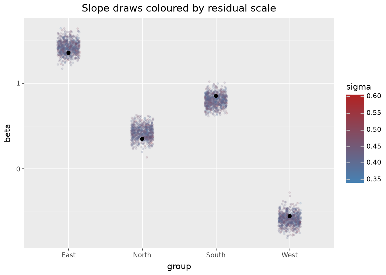
Request beta[groups] and the scalar sigma together: sigma is broadcast onto every beta[groups] row, so you can colour one by the other directly.

mixed = td.parameter_draws(dt, "beta", "sigma")

Cross-join detected between frame 0 and 1. Broadcasting scalar or differently-dimensioned variable on dims ['chain', 'draw'].

(
    lp.ggplot(mixed.to_pandas(), lp.aes("groups", "beta"))
    + lp.geom_jitter(lp.aes(color="sigma"), width=0.15, alpha=0.15, size=0.8)
    + lp.geom_point(
        data=truth.to_pandas(),
        mapping=lp.aes("groups", "beta_true"),
        color="black",
        size=2.0,
    )
    + lp.scale_color_gradient(low="steelblue", high="firebrick")
    + lp.labs(
        x="group",
        y="beta",
        color="sigma",
        title="Slope draws coloured by residual scale",
    )
)

Posterior slopes by group, coloured by each draw’s residual sigma.

(
    p9.ggplot(mixed.to_pandas(), p9.aes("groups", "beta"))
    + p9.geom_jitter(p9.aes(color="sigma"), width=0.15, alpha=0.15, size=0.8)
    + p9.geom_point(
        data=truth.to_pandas(),
        mapping=p9.aes("groups", "beta_true"),
        color="black",
        size=2.0,
    )
    + p9.scale_color_gradient(low="steelblue", high="firebrick")
    + p9.labs(
        x="group",
        y="beta",
        color="sigma",
        title="Slope draws coloured by residual scale",
    )
)

Next, compare fitted posterior draws with model priors using compare_draws().