Prediction space

Fit a PyMC model, join posterior expectations to covariates with prediction_draws(), and plot them

prediction_draws() joins posterior prediction draws such as mu to covariates, producing one tidy row per chain × draw × observation. Parameters are deliberately excluded — prediction space stays separate from parameter space, so coefficients never get duplicated across observations.

Pass a DataFrame when you want explicit control over the covariates used for plotting. With newdata=None, prediction_draws() reads covariates from a constant-data group in the ArviZ object and fails loudly if that group is missing.

Full PyMC workflow

The workflow starts from observed data with strong group differences, fits a PyMC model, asks PyMC for posterior expectations mu[obs_ind], and then uses prediction_draws() to attach those draws to x, groups, and observed y.

Code

from pathlib import Path
import sys

import polars as pl
import pymc as pm
import tidydraws as td
import lets_plot as lp
import plotnine as p9

for parent in [Path.cwd(), *Path.cwd().parents]:
    helper_dir = parent / "docs" / "examples"
    if (helper_dir / "_pymc_workflow.py").exists():
        sys.path.insert(0, str(helper_dir))
        break

from tidydraws import point_interval
from _pymc_workflow import simulate_grouped_regression

lp.LetsPlot.setup_html()

workflow = simulate_grouped_regression(seed=2026)
observed = workflow.observed

coords = {
    "groups": workflow.group_names,
    "obs_ind": observed.get_column("obs_ind").to_numpy(),
}

Build our PyMC model and fit.

with pm.Model(coords=coords) as model:
    x = pm.Data("x", observed.get_column("x").to_numpy(), dims="obs_ind")
    group_idx = pm.Data(
        "group_idx",
        observed.get_column("group_idx").to_numpy().astype("int64"),
        dims="obs_ind",
    )
    intercept = pm.Normal("intercept", mu=0.0, sigma=2.0, dims="groups")
    beta = pm.Normal("beta", mu=0.0, sigma=1.5, dims="groups")
    sigma = pm.HalfNormal("sigma", sigma=1.0)
    mu = pm.Deterministic(
        "mu",
        intercept[group_idx] + beta[group_idx] * x,
        dims="obs_ind",
    )
    pm.Normal(
        "y",
        mu=mu,
        sigma=sigma,
        observed=observed.get_column("y").to_numpy(),
        dims="obs_ind",
    )
    dt = pm.sample(
        draws=400,
        tune=400,
        random_seed=2027,
    )
    pm.sample_posterior_predictive(
        dt,
        var_names=["mu", "y"],
        predictions=True,
        extend_inferencedata=True,
        random_seed=2028,
        progressbar=False,
    )

Initializing NUTS using jitter+adapt_diag...
Multiprocess sampling (2 chains in 2 jobs)
NUTS: [intercept, beta, sigma]
/home/runner/work/tidydraws/tidydraws/.venv/lib/python3.12/site-packages/pymc/step_methods/hmc/quadpotential.py:321: RuntimeWarning: overflow encountered in dot

Sampling 2 chains for 400 tune and 400 draw iterations (800 + 800 draws total) took 1 seconds.
We recommend running at least 4 chains for robust computation of convergence diagnostics
The rhat statistic is larger than 1.01 for some parameters. This indicates problems during sampling. See https://arxiv.org/abs/1903.08008 for details
Sampling: [y]

dt

Use tidydraws

One call joins mu to the observed covariates and responses:

pred = td.prediction_draws(dt, newdata=observed, var_name="mu")
pred.head()

shape: (5, 9)

chain	draw	obs_ind	mu	groups	group_idx	x	mu_true	y
i64	i64	i64	f64	str	i64	f64	f64	f64
0	0	0	-2.038775	"North"	0	-2.06345	-1.972207	-2.106032
0	0	1	-1.929716	"North"	0	-1.806841	-1.882394	-1.794667
0	0	2	-1.928457	"North"	0	-1.80388	-1.881358	-2.253447
0	0	3	-1.742612	"North"	0	-1.366599	-1.72831	-2.094702
0	0	4	-1.694453	"North"	0	-1.253284	-1.688649	-2.373679

Note the columns: chain, draw, obs_ind, mu, groups, group_idx, x, mu_true, and y. No beta, no intercept — parameters stay in their own frame.

Plotting

Posterior expected fit by group

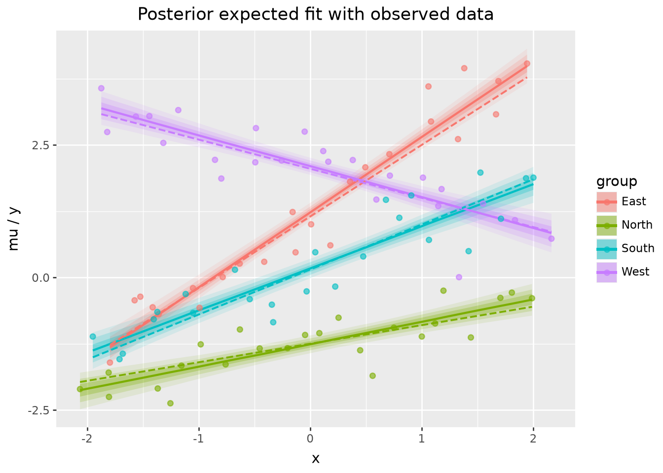
Summarise mu per observation with 50%, 80%, and 95% intervals, then draw nested ribbons, a median line, the true generating line, and the raw observed y values.

summary = td.point_interval(
    pred,
    "mu",
    group_by=["obs_ind", "x", "groups", "mu_true", "y"],
    probs=(0.50, 0.80, 0.95),
).sort(["groups", "x"])
fit_median = summary
observed_points = (
    summary.select("x", "y", "groups", "mu_true").unique().sort(["groups", "x"])
)

(
    lp.ggplot(summary.to_pandas(), lp.aes("x"))
    + lp.geom_ribbon(
        mapping=lp.aes(
            ymin="mu_lower_0.95",
            ymax="mu_upper_0.95",
            fill=lp.as_discrete("groups"),
            group="groups",
        ),
        alpha=0.10,
        color="transparent",
    )
    + lp.geom_ribbon(
        mapping=lp.aes(
            ymin="mu_lower_0.80",
            ymax="mu_upper_0.80",
            fill=lp.as_discrete("groups"),
            group="groups",
        ),
        alpha=0.18,
        color="transparent",
    )
    + lp.geom_ribbon(
        mapping=lp.aes(
            ymin="mu_lower_0.50",
            ymax="mu_upper_0.50",
            fill=lp.as_discrete("groups"),
            group="groups",
        ),
        alpha=0.28,
        color="transparent",
    )
    + lp.geom_line(
        mapping=lp.aes(y="mu", color=lp.as_discrete("groups")),
        size=0.9,
    )
    + lp.geom_line(
        data=observed_points.to_pandas(),
        mapping=lp.aes(y="mu_true", color=lp.as_discrete("groups")),
        linetype="dashed",
        size=0.8,
    )
    + lp.geom_point(
        data=observed_points.to_pandas(),
        mapping=lp.aes(y="y", color=lp.as_discrete("groups")),
        size=1.8,
        alpha=0.6,
    )
    + lp.labs(
        x="x",
        y="mu / y",
        color="group",
        fill="group",
        title="Posterior expected fit with observed data",
    )
)

Posterior expected fit by group with nested credible ribbons, true lines, and observed data.

(
    p9.ggplot(summary.to_pandas(), p9.aes("x"))
    + p9.geom_ribbon(
        mapping=p9.aes(
            ymin="mu_lower_0.95",
            ymax="mu_upper_0.95",
            fill="groups",
            group="groups",
        ),
        alpha=0.10,
    )
    + p9.geom_ribbon(
        mapping=p9.aes(
            ymin="mu_lower_0.80",
            ymax="mu_upper_0.80",
            fill="groups",
            group="groups",
        ),
        alpha=0.18,
    )
    + p9.geom_ribbon(
        mapping=p9.aes(
            ymin="mu_lower_0.50",
            ymax="mu_upper_0.50",
            fill="groups",
            group="groups",
        ),
        alpha=0.28,
    )
    + p9.geom_line(
        mapping=p9.aes(y="mu", color="groups"),
        size=0.9,
    )
    + p9.geom_line(
        data=observed_points.to_pandas(),
        mapping=p9.aes(y="mu_true", color="groups"),
        linetype="dashed",
        size=0.8,
    )
    + p9.geom_point(
        data=observed_points.to_pandas(),
        mapping=p9.aes(y="y", color="groups"),
        size=1.8,
        alpha=0.6,
    )
    + p9.labs(
        x="x",
        y="mu / y",
        color="group",
        fill="group",
        title="Posterior expected fit with observed data",
    )
)

Posterior predicted fit by group

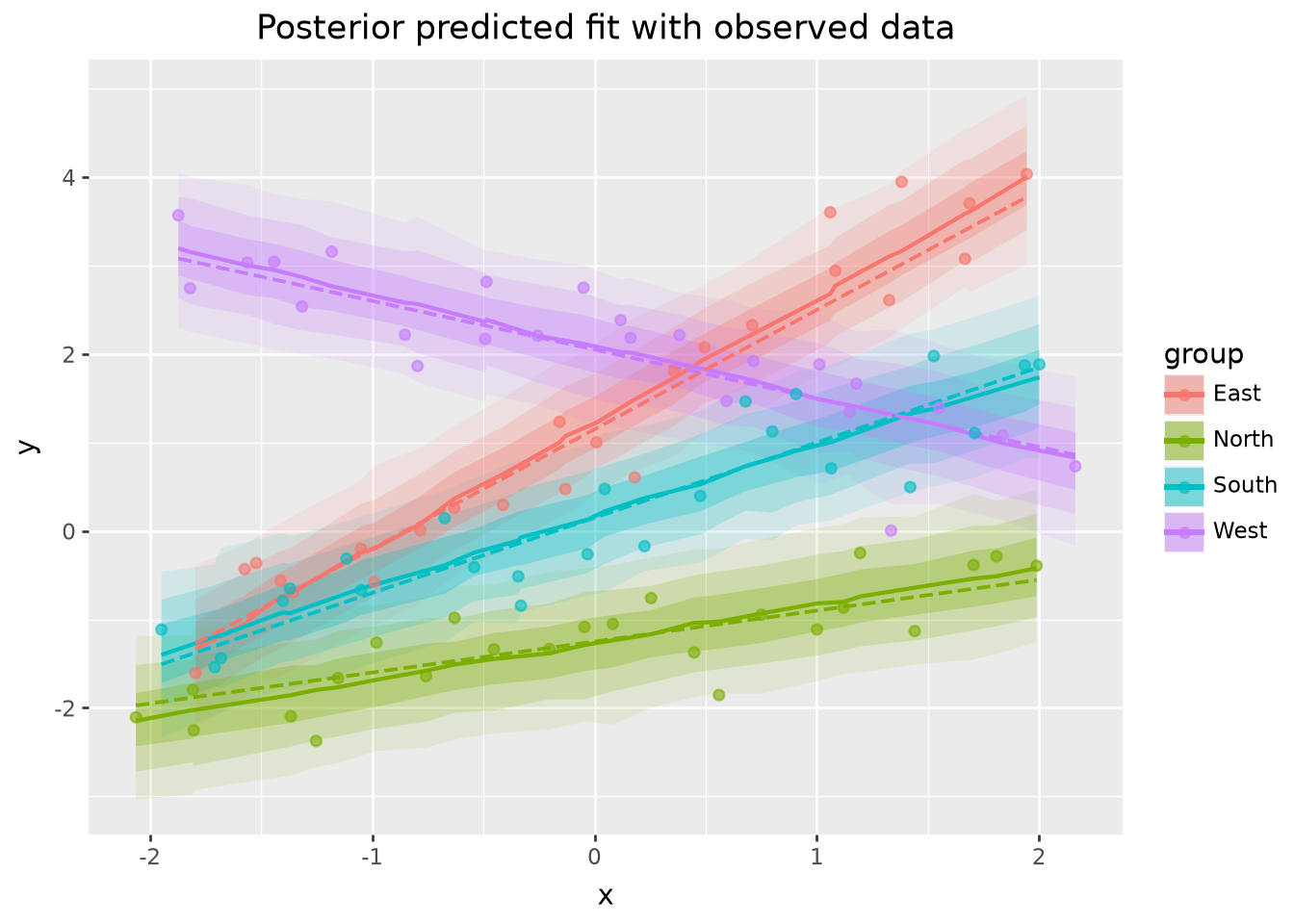
The same interval plot, now using posterior predictive draws of the observed outcome \(y\) rather than the posterior expectation \(\mu\). Because \(y\) includes the observation noise (\(\sigma\)), the intervals are wider — they represent the distribution of new data, not the mean.

Code

pred_y = td.prediction_draws(dt, newdata=observed, var_name="y").rename({
    "y_right": "y_obs"
})

summary_y = td.point_interval(
    pred_y,
    "y",
    group_by=["obs_ind", "x", "groups", "mu_true", "y_obs"],
    probs=(0.50, 0.80, 0.95),
).sort(["groups", "x"])

(
    lp.ggplot(summary_y.to_pandas(), lp.aes("x"))
    + lp.geom_ribbon(
        mapping=lp.aes(
            ymin="y_lower_0.95",
            ymax="y_upper_0.95",
            fill=lp.as_discrete("groups"),
            group="groups",
        ),
        alpha=0.10,
        color="transparent",
    )
    + lp.geom_ribbon(
        mapping=lp.aes(
            ymin="y_lower_0.80",
            ymax="y_upper_0.80",
            fill=lp.as_discrete("groups"),
            group="groups",
        ),
        alpha=0.18,
        color="transparent",
    )
    + lp.geom_ribbon(
        mapping=lp.aes(
            ymin="y_lower_0.50",
            ymax="y_upper_0.50",
            fill=lp.as_discrete("groups"),
            group="groups",
        ),
        alpha=0.28,
        color="transparent",
    )
    + lp.geom_line(
        mapping=lp.aes(y="y", color=lp.as_discrete("groups")),
        size=0.9,
    )
    + lp.geom_line(
        data=observed_points.to_pandas(),
        mapping=lp.aes(y="mu_true", color=lp.as_discrete("groups")),
        linetype="dashed",
        size=0.8,
    )
    + lp.geom_point(
        data=observed_points.to_pandas(),
        mapping=lp.aes(y="y", color=lp.as_discrete("groups")),
        size=1.8,
        alpha=0.6,
    )
    + lp.labs(
        x="x",
        y="y",
        color="group",
        fill="group",
        title="Posterior predicted fit with observed data",
    )
)

Posterior predicted fit by group with nested credible intervals, true lines, and observed data.

(
    p9.ggplot(summary_y.to_pandas(), p9.aes("x"))
    + p9.geom_ribbon(
        mapping=p9.aes(
            ymin="y_lower_0.95",
            ymax="y_upper_0.95",
            fill="groups",
            group="groups",
        ),
        alpha=0.10,
    )
    + p9.geom_ribbon(
        mapping=p9.aes(
            ymin="y_lower_0.80",
            ymax="y_upper_0.80",
            fill="groups",
            group="groups",
        ),
        alpha=0.18,
    )
    + p9.geom_ribbon(
        mapping=p9.aes(
            ymin="y_lower_0.50",
            ymax="y_upper_0.50",
            fill="groups",
            group="groups",
        ),
        alpha=0.28,
    )
    + p9.geom_line(
        mapping=p9.aes(y="y", color="groups"),
        size=0.9,
    )
    + p9.geom_line(
        data=observed_points.to_pandas(),
        mapping=p9.aes(y="mu_true", color="groups"),
        linetype="dashed",
        size=0.8,
    )
    + p9.geom_point(
        data=observed_points.to_pandas(),
        mapping=p9.aes(y="y", color="groups"),
        size=1.8,
        alpha=0.6,
    )
    + p9.labs(
        x="x",
        y="y",
        color="group",
        fill="group",
        title="Posterior predicted fit with observed data",
    )
)

Group-specific panels

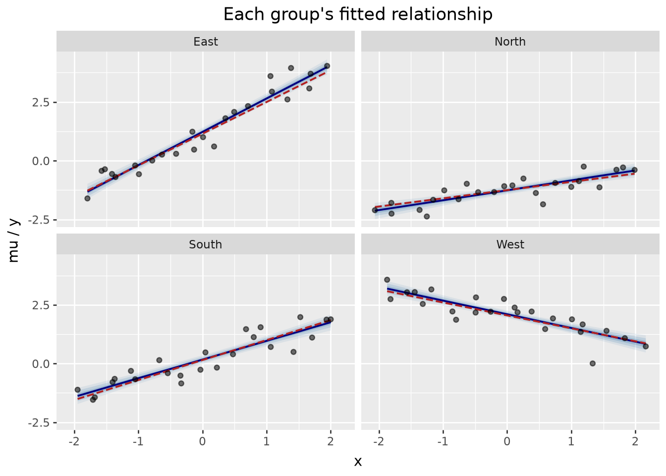
Faceting is optional; the tidy frame already contains the group label needed by any plotting backend.

(
    lp.ggplot(summary.to_pandas(), lp.aes("x"))
    + lp.geom_ribbon(
        mapping=lp.aes(ymin="mu_lower_0.95", ymax="mu_upper_0.95", group="groups"),
        fill="steelblue",
        alpha=0.10,
        color="transparent",
    )
    + lp.geom_ribbon(
        mapping=lp.aes(ymin="mu_lower_0.80", ymax="mu_upper_0.80", group="groups"),
        fill="steelblue",
        alpha=0.18,
        color="transparent",
    )
    + lp.geom_ribbon(
        mapping=lp.aes(ymin="mu_lower_0.50", ymax="mu_upper_0.50", group="groups"),
        fill="steelblue",
        alpha=0.28,
        color="transparent",
    )
    + lp.geom_line(mapping=lp.aes(y="mu"), color="navy", size=0.8)
    + lp.geom_line(
        data=observed_points.to_pandas(),
        mapping=lp.aes(y="mu_true"),
        color="firebrick",
        linetype="dashed",
        size=0.8,
    )
    + lp.geom_point(
        data=observed_points.to_pandas(),
        mapping=lp.aes(y="y"),
        color="black",
        size=1.6,
        alpha=0.55,
    )
    + lp.facet_wrap(facets="groups", ncol=2)
    + lp.labs(x="x", y="mu / y", title="Each group's fitted relationship")
)

Posterior expected fit faceted by group.

(
    p9.ggplot(summary.to_pandas(), p9.aes("x"))
    + p9.geom_ribbon(
        mapping=p9.aes(ymin="mu_lower_0.95", ymax="mu_upper_0.95", group="groups"),
        fill="steelblue",
        alpha=0.10,
    )
    + p9.geom_ribbon(
        mapping=p9.aes(ymin="mu_lower_0.80", ymax="mu_upper_0.80", group="groups"),
        fill="steelblue",
        alpha=0.18,
    )
    + p9.geom_ribbon(
        mapping=p9.aes(ymin="mu_lower_0.50", ymax="mu_upper_0.50", group="groups"),
        fill="steelblue",
        alpha=0.28,
    )
    + p9.geom_line(mapping=p9.aes(y="mu"), color="navy", size=0.8)
    + p9.geom_line(
        data=observed_points.to_pandas(),
        mapping=p9.aes(y="mu_true"),
        color="firebrick",
        linetype="dashed",
        size=0.8,
    )
    + p9.geom_point(
        data=observed_points.to_pandas(),
        mapping=p9.aes(y="y"),
        color="black",
        size=1.6,
        alpha=0.55,
    )
    + p9.facet_wrap("~groups", ncol=2)
    + p9.labs(x="x", y="mu / y", title="Each group's fitted relationship")
)

Spaghetti posterior expectation lines

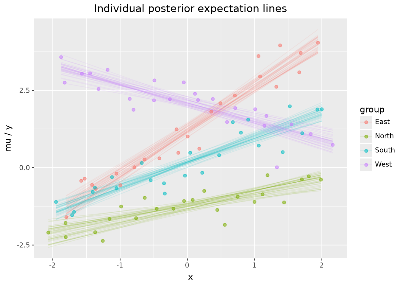
Intervals summarise the draw distribution. Spaghetti lines show individual posterior expectation draws directly; here the first 40 (chain, draw) pairs are plotted for stability.

draw_ids = (
    pred
    .select("chain", "draw")
    .unique()
    .sort(["chain", "draw"])
    .head(40)
    .with_row_index("curve_id")
)
spaghetti = (
    pred
    .join(draw_ids, on=["chain", "draw"], how="inner")
    .with_columns(
        (pl.col("groups") + "_" + pl.col("curve_id").cast(pl.Utf8)).alias("curve")
    )
    .sort(["curve", "x"])
)

(
    lp.ggplot(spaghetti.to_pandas(), lp.aes("x"))
    + lp.geom_line(
        lp.aes(y="mu", group="curve", color=lp.as_discrete("groups")),
        alpha=0.10,
        size=0.5,
    )
    + lp.geom_point(
        data=observed_points.to_pandas(),
        mapping=lp.aes(y="y", color=lp.as_discrete("groups")),
        size=1.7,
        alpha=0.55,
    )
    + lp.labs(
        x="x", y="mu / y", color="group", title="Individual posterior expectation lines"
    )
)

(
    p9.ggplot(spaghetti.to_pandas(), p9.aes("x"))
    + p9.geom_line(p9.aes(y="mu", group="curve", color="groups"), alpha=0.10, size=0.5)
    + p9.geom_point(
        data=observed_points.to_pandas(),
        mapping=p9.aes(y="y", color="groups"),
        size=1.7,
        alpha=0.55,
    )
    + p9.labs(
        x="x", y="mu / y", color="group", title="Individual posterior expectation lines"
    )
)

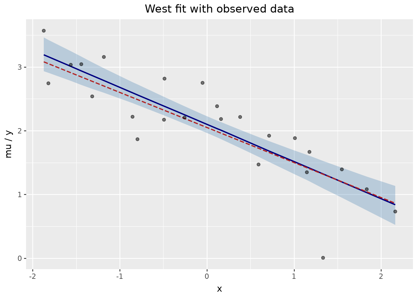
Filter before plotting

Subset with .filter() before summarising — useful when the full prediction space is large.

west = td.prediction_draws(dt, newdata=observed, var_name="mu").filter(
    pl.col("groups") == "West"
)
s_west = td.point_interval(
    west, "mu", group_by=["obs_ind", "x", "y", "mu_true"], probs=(0.89,)
).sort("x")

(
    lp.ggplot(s_west.to_pandas(), lp.aes("x"))
    + lp.geom_ribbon(
        lp.aes(ymin="mu_lower", ymax="mu_upper"),
        fill="steelblue",
        alpha=0.3,
        color="transparent",
    )
    + lp.geom_line(lp.aes(y="mu"), color="navy", size=0.9)
    + lp.geom_line(lp.aes(y="mu_true"), color="firebrick", linetype="dashed", size=0.8)
    + lp.geom_point(lp.aes(y="y"), color="black", size=1.6, alpha=0.5)
    + lp.labs(x="x", y="mu / y", title="West fit with observed data")
)

(
    p9.ggplot(s_west.to_pandas(), p9.aes("x"))
    + p9.geom_ribbon(
        p9.aes(ymin="mu_lower", ymax="mu_upper"),
        fill="steelblue",
        alpha=0.3,
    )
    + p9.geom_line(p9.aes(y="mu"), color="navy", size=0.9)
    + p9.geom_line(p9.aes(y="mu_true"), color="firebrick", linetype="dashed", size=0.8)
    + p9.geom_point(p9.aes(y="y"), color="black", size=1.6, alpha=0.5)
    + p9.labs(x="x", y="mu / y", title="West fit with observed data")
)

See parameter_draws() for parameter space, or compare_draws() for prior vs posterior.